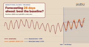
A store needs to know its sales for the next 28 days to order stock and schedule staff. The data is a single column of daily sales over three years. This is a time series forecasting problem. What sets it apart from the earlier machine learning problems is that the data is ordered, so every step (splitting, feature engineering, evaluation) must respect the arrow of time. This article goes from simple baselines, through ARIMA and SARIMA, to gradient boosting with lag features, on 1,096 days of simulated data, with real output and with the results that did not turn out as predicted.
It follows Anomaly detection in transactions: Isolation Forest and autoencoders, where transactions were treated as independent; here that assumption no longer holds. The gradient boosting part reuses LightGBM from Gradient boosting with XGBoost and LightGBM: when it beats deep learning and the metric selection from Model evaluation for classifiers: precision, recall, ROC and imbalanced data. Environment for re-running: Apple M4, 16 GB, CPU, Python 3.10, pandas 2.0.2, NumPy 1.25.0, scikit-learn 1.3.0, statsmodels 0.14.0, LightGBM 3.3.5. The time series is entirely simulated, not real sales.
A simulated sales time series
We generate a daily sales time series from January 1, 2020 to December 31, 2022 by multiplying several components: a steady upward trend (100 plus 0.08 per day), a weekly seasonality (Saturday and Sunday 25 to 30% higher), a yearly seasonality (15% swing), promotions on the 15th and the last day of each month (a 35% lift), and Gaussian noise. This is a familiar shape for retail data, and because we know the generating formula we can check which model learns which part.
trend = 100 + 0.08 * t
promo = ((idx.day.to_numpy() == 15) | idx.is_month_end).astype(int)
sales = trend * weekly * yearly * (1 + 0.35 * promo) + noise
s = pd.Series(sales.round(1), index=idx, name=sales_million)
[Data] 1096 days, from 2020-01-01 to 2022-12-31
count    1096.0
mean      155.7
std        41.1
min        72.5
25%       125.0
50%       151.6
75%       180.1
max       346.9
Time series evaluation: never shuffle the data
When evaluating a time series, rule number one is that the test data must come after the training data. The book Forecasting: Principles and Practice by Hyndman and Athanasopoulos describes the rolling forecasting origin procedure: each training set contains only observations before the test point, and the errors are then averaged over many cut points. In scikit-learn, TimeSeriesSplit does the same thing: at split k, the training set is the first k blocks and the test set is block k+1, so each training set is a superset of the previous one; the test_size parameter fixes the test length and gap leaves a gap between the two sets.
For time series metrics, besides MAE, RMSE and MAPE, we use MASE (mean absolute scaled error). According to the same book, MASE divides the error by the MAE of a baseline method (here seasonal naive with period m = 7) computed on the training set, so it is unit-free: a MASE below 1 means better than the average seasonal naive error on the training data itself. MAPE gets distorted when some days have sales near 0, while MASE does not have that problem.
Time series baselines: the four simplest methods
Also according to the simple methods chapter by Hyndman and Athanasopoulos, there are four baselines: mean (every forecast equals the historical average), naive (equals the last value), seasonal naive (equals the value from the same point of the previous cycle, for example the same weekday last week) and drift (the straight line from the first to the last observation, extended forward). Each baseline for a time series takes only a few lines of NumPy:
out["Mean"] = np.full(h, train.mean())
out["Naive"] = np.full(h, train.iloc[-1])
out["Seasonal naive (m=7)"] = np.tile(train.iloc[-7:].to_numpy(), h // 7 + 1)[:h]
out["Drift"] = train.iloc[-1] + np.arange(1, h + 1) * (train.iloc[-1] - train.iloc[0]) / (len(train) - 1)
Baselines are the honest yardstick when forecasting a time series: a model that does not beat seasonal naive does not deserve to go into production. With data that has a clear weekly seasonality, like retail sales, seasonal naive is a formidable opponent, and we will see it beat several "fancier" models.
ARIMA for time series: stationarity, differencing and seasonality
ARIMA(p, d, q) combines three things: autoregression of order p (the current value depends on the previous p values), differencing of order d to make the series stationary, and a moving average of order q over the errors. According to the statsmodels documentation, the order parameter is the tuple (p, d, q) and seasonal_order is the tuple (P, D, Q, s), where s is the seasonal period (it must be greater than 1). Before choosing d, we check the stationarity of the time series with the augmented Dickey-Fuller (ADF) test, whose null hypothesis is that the series has a unit root (non-stationary):
[ADF on the original series] p-value = 0.3130
[ADF after first-order differencing] p-value = 1.71e-07
[ADF after seasonal differencing at lag 7] p-value = 1.16e-03
The original series has a p-value of 0.313: we cannot reject the non-stationarity hypothesis, as expected for a series with an upward trend. After first-order differencing the p-value drops to 1.71e-07: the series is stationary, so d = 1. We try two ARIMA models for this time series at the cut point of December 3, 2022 (train 1,068 days, forecast the next 28 days): ARIMA(2, 1, 2) without seasonality and SARIMA(1, 1, 1)(1, 1, 1, 7) with weekly seasonality. In code, ARIMA is just one line:
from statsmodels.tsa.arima.model import ARIMA
from statsmodels.tsa.statespace.sarimax import SARIMAX
arima = ARIMA(train, order=(2, 1, 2)).fit().forecast(28)
sarima = SARIMAX(train, order=(1, 1, 1), seasonal_order=(1, 1, 1, 7)).fit(disp=False).forecast(28)
Time series forecast results at a single cut point
[Single cut point] train up to 2022-12-03 (1068 days), test 2022-12-04 → 2022-12-31 (28 days), running all models took 4.4 seconds
  MASE denominator = seasonal naive m=7 MAE on train = 13.34
  model | MAE | RMSE | MAPE% | MASE
  LightGBM (calendar + lag ≥ 28)   9.81   12.52   5.52  0.735
  SARIMAX + promo variable        10.08   12.88   5.65  0.756
  SARIMA(1,1,1)(1,1,1,7)          10.30   19.66   5.22  0.773
  Seasonal naive (m=7)            20.45   34.08  11.71  1.534
  ARIMA(2,1,2)                    25.35   32.36  14.12  1.901
  Mean                            26.42   37.72  13.46  1.981
  Naive (last value)              34.31   40.24  21.43  2.573
  Drift                           34.87   40.95  21.89  2.615
Three points deserve a careful read. First, non-seasonal ARIMA (MASE 1.901) loses even to seasonal naive (1.534): it ignores the weekly cycle, and multi-step ARIMA forecasts converge to a nearly flat line. Once a seasonal component is added, SARIMA drops the MASE to 0.773. Second, naive and drift are the worst (MASE above 2.5) because weekend and weekday sales differ by up to 30%, so the "last value" depends on which weekday the final day of the train set falls on. Third, the top three models differ very little (0.735, 0.756, 0.773), and over just 28 days that difference is within the noise; we need many cut points to draw a conclusion.
Gradient boosting for time series: calendar and lag features
Decision trees have no notion of time, so we have to turn the time series into a table: each row is a day and the columns are features. Two groups are useful: calendar features (day of week, day of month, month, promotion day) and lag features (earlier values of the series itself, rolling averages). The vital condition is that every lag must be greater than or equal to the forecast horizon. To forecast 28 days, we may only use lags of 28 days or more, because when forecasting day 20 we do not yet know the sales of day 19:
def make_features(series, min_lag=28):
    d = pd.DataFrame({"y": series})
    d["dow"] = d.index.dayofweek
    d["dom"] = d.index.day
    d["month"] = d.index.month
    d["is_promo"] = ((d.index.day == 15) | d.index.is_month_end).astype(int)
    d["lag28"] = d["y"].shift(min_lag)
    d["lag35"] = d["y"].shift(min_lag + 7)
    d["roll28_28"] = d["y"].shift(min_lag).rolling(28).mean()
    return d
This way of forecasting a time series is called direct forecasting: one model for the whole horizon, instead of forecasting step by step and feeding the results back in as lags (recursive), which tends to accumulate errors. The LightGBM importance (gain) shows that the model relies mainly on lags, as expected, because lag28 and lag35 fall on the same weekday as the day being forecast:
  LightGBM importance (gain, % of total):
lag28        48.6
lag35        31.6
is_promo     10.0
month         5.1
roll28_28     2.3
dow           1.7
dom           0.7
is_promo accounts for 10%: the trees pick up the promotion effect that plain ARIMA lacks. To be fair, we also add a SARIMAX model with exog set to the promotion variable (known in advance for the future, like a company's promotion calendar). This model reaches an MAE of 10.08, close to LightGBM (9.81): when ARIMA gets the same information, the gap narrows considerably.
Rolling origin: evaluating a time series over 11 cut points
A single cut point is not enough to draw conclusions about time series forecasting. We repeat the whole procedure (retraining from scratch at each point) for the 11 month-end cut points from January 31, 2022 to November 30, 2022, forecasting 28 days each time, then take the average MASE:
[Rolling origin] 11 cut points (end of January → November 2022), 28-day forecast each; mean MASE ± standard deviation
  (total time 32 seconds)
  LightGBM (calendar + lag ≥ 28)  0.610 ± 0.127 | best 0.43, worst 0.76
  SARIMAX + promo variable        0.680 ± 0.251 | best 0.42, worst 1.35
  SARIMA(1,1,1)(1,1,1,7)          1.107 ± 0.391 | best 0.59, worst 1.95
  Seasonal naive (m=7)            1.439 ± 0.268 | best 1.04, worst 1.87
  ARIMA(2,1,2)                    1.975 ± 0.302 | best 1.51, worst 2.53
  Mean                            3.232 ± 1.204 | best 1.74, worst 4.99
  Naive (last value)              4.635 ± 2.881 | best 1.80, worst 10.91
  Drift                           4.784 ± 2.973 | best 1.84, worst 11.21
The picture is much clearer when forecasting a time series over many cut points. LightGBM has a mean MASE of 0.610 and is stable (standard deviation 0.127, worst 0.76). SARIMAX with promotions is close on average (0.680) but fluctuates twice as much (standard deviation 0.251) and has a cut point as bad as 1.35.
Plain SARIMA (1.107) beats seasonal naive (1.439) on average but fluctuates strongly (standard deviation 0.391, with a cut point as bad as 1.95, worse than even seasonal naive's worst of 1.87). The cause lies in the promotion days (the 15th and month end, where sales jump 35%) that a period-7 SARIMA does not know about. We verify this by pooling the daily absolute errors across the 11 cut points and separating promotion days from regular days:
[Error by day type, pooled over 11 cut points] MAE on promotion days (15th and month end) vs regular days:
  SARIMA(1,1,1)(1,1,1,7)         promo  55.82 (n=12) | regular  12.81 (n=296) | ratio 4.36
  SARIMAX + promo variable       promo  11.75 (n=12) | regular   8.75 (n=296) | ratio 1.34
  LightGBM (calendar + lag ≥ 28) promo  13.95 (n=12) | regular   7.68 (n=296) | ratio 1.82
  Seasonal naive (m=7)           promo  59.28 (n=12) | regular  17.11 (n=296) | ratio 3.46
  SARIMA errors (unaware of promotions) by cut point, MASE per point:
  0.88 0.59 0.82 0.90 1.03 1.38 1.95 1.42 1.53 0.91 0.77
SARIMA is off by 4.36 times as much on promotion days (MAE 55.82 vs 12.81), while SARIMAX with the promotion variable is off by only 1.34 times. This is direct evidence for the explanation above, but not the whole story: the promotion sample is small (12 days: each 28-day window contains exactly one 15th, and the February window also contains the 28th), and even on regular days SARIMA (12.81) is worse than SARIMAX (8.75), so noise in estimating the seasonal parameters also contributes. The worst cut point (MASE 1.95) is the end of July; this article does not dig into that one point. This is also simulated data in which we set a strong promotion effect ourselves; on real data, the gap between model families is usually narrower.
Time series pitfalls: lags and cross-validation
Future leakage through short lags
Try using lag7 for the 28-day time series forecasting problem, and to forecast we take lag7 from the real 28 test days themselves (impossible in real life, because the sales of day 21 do not exist yet at that time):
[Future leakage] LightGBM uses lag7 but takes the lag from the real 28 test days themselves:
  MAE = 8.84, MASE = 0.662  (vs the correct approach, lag ≥ 28: MAE = 9.81)
The result looks "better" (MAE 8.84 vs 9.81), but only by about 10% in this experiment. The difference is small because the simulated data has a very regular weekly seasonality, so lag28 already contains almost all the information that lag7 has. Do not take leakage lightly because of this: on data with short-term shocks or strong autocorrelation, leaked short lags can make a model look falsely good, and you only find out at deployment.
Shuffled KFold vs TimeSeriesSplit
[CV on train, same LightGBM model with lag ≥ 28]
  Shuffled KFold  : MAE = 6.64 ± 0.45
  TimeSeriesSplit : MAE = 7.06 ± 1.30 (per fold: [9.17 6.19 7.46 7.18 5.29])
  Real MAE on the 28 test days after the cut point: 9.81
Shuffled KFold gives an MAE of 6.64, more optimistic than TimeSeriesSplit (7.06), and both are more optimistic than the real MAE after the cut point (9.81). The difference between the two CV methods is small here because we used lag ≥ 28, so the features do not leak, and the series has only a mild linear trend. Even so, shuffled KFold gives a much lower standard deviation (0.45 vs 1.30), meaning it hides some of the real uncertainty. The safe rule: use only TimeSeriesSplit or rolling origin, and do not trust a single CV number as a forecast of the future.
Trees do not extrapolate trends
A tree model forecasts a time series with the average of the leaves it saw during training, so it cannot go beyond the old range of values. We verify this by training only on 2020 to 2021 with calendar features, then forecasting all of 2022:
[Trend] average sales for 2020 → 2022: 124.1 → 187.3
  LightGBM with calendar features only, train 2020-2021, forecast all of 2022: mean forecast = 142.5, actual = 187.3
Real sales rose from 124.1 to 187.3, and the model forecast only about 142.5 for 2022, 24% below actual, because it had never seen sales levels that high. Lags "carry" the current level into the features, so a model with lags (as above) suffers less from this problem; but with a strong trend, you should detrend (forecast the difference from the lag) or combine with a model that has an explicit trend.
Comparing three families of time series forecasting methods
| Criterion | Baseline | ARIMA / SARIMA(X) | Gradient boosting |
|---|---|---|---|
| Setup effort | A few lines | Choose (p,d,q)(P,D,Q,s), test stationarity | Design lag and calendar features |
| Seasonality | Seasonal naive | Yes, via seasonal_order | Via calendar and lag features |
| Exogenous variables (promotions) | No | SARIMAX, exog | Add a column, easy |
| Trend | Drift | Yes, via differencing | Does not extrapolate |
| MASE in this article (rolling) | 1.439 (seasonal naive) | 1.107 (SARIMA), 0.680 (with exog) | 0.610 |
| Stability (standard deviation) | 0.268 | 0.391 / 0.251 | 0.127 |
When not to use gradient boosting for a time series
- Short time series: with a few dozen points, ARIMA or exponential smoothing is much more stable than trees.
- You need proper prediction intervals for the time series: ARIMA gives forecast intervals from a probabilistic model; LightGBM needs quantile regression or conformal prediction on top.
- Strong, long-lasting trends: trees do not extrapolate, as in the 142.5 vs 187.3 example.
- Thousands of small time series: retraining each series separately is costly to operate; consider a global model or baselines.
Common time series forecasting mistakes
- Random splits (
train_test_split, shuffled KFold): future data leaks into training; always split by time. - Using lags shorter than the horizon: at real forecast time, that lag does not exist yet.
- Skipping baselines for the time series: ARIMA(2,1,2) in this article even lost to seasonal naive at a single cut point.
- Concluding from a single cut point: SARIMA's MASE ranged from 0.59 to 1.95 across 11 points.
- Choosing d and D by gut feeling: run the ADF test and look at the plots; do not over-difference.
- Forgetting to retrain periodically: a time series changes its pattern after shocks, and promotion changes or holiday seasons make the model stale.
Checklist
- For a time series, always start with the four baselines and report MASE alongside MAE.
- Split the time series and cross-validate by time, using many cut points.
- Check stationarity of the time series with ADF, choose d, and add seasonal_order when there is a cycle.
- With gradient boosting, keep every lag greater than or equal to the horizon, and add calendar features and known-in-advance exogenous variables.
- Test tree models on time series with a strong trend, and consider detrending.
- Monitor time series forecast error after deployment and retrain periodically.
The full source code is in code/s7-18 (forecast_demo.py, output.txt, requirements.txt), run with python forecast_demo.py. All figures are real output from an Apple M4, 16 GB, CPU, with a fixed seed (the rolling origin run takes about 32 seconds). We set the promotion effect ourselves, so the model ranking does not generalize to real time series.
Next article
Building a product recommender in Python: content-based and collaborative filtering. After forecasting total sales, the next article goes down to the individual customer level: recommending which products to buy next with content-based and collaborative filtering.