Among 60,300 transactions from an online store, only 300 (0.5%) are anomalous: a large amount at midnight, an order shipped very far from the usual address, dozens of purchases packed into 24 hours. Nobody has labeled them. This is the classic anomaly detection problem: find the observations that differ sharply from the rest when you have almost no labels. This article compares three approaches to anomaly detection, Isolation Forest, Local Outlier Factor (LOF) and a PyTorch autoencoder, on synthetic data, with real output and with the results that did not match expectations.
It continues Customer clustering: K-Means, DBSCAN and dimensionality reduction with PCA, where DBSCAN's noise label was already a rudimentary form of anomaly detection, and it reuses the metrics from Model evaluation for classifiers: precision, recall, ROC and imbalanced data. Environment for rerunning: Apple Silicon machine with 16 GB, CPU, Python 3.11, scikit-learn 1.2.2, PyTorch 2.0.1, NumPy 1.24.3. The data is entirely synthetic, not real transactions.
The anomaly detection problem and why it is hard
According to the scikit-learn Novelty and Outlier Detection documentation, there are two situations to tell apart. Outlier detection (unsupervised): the training data already contains outliers, and the model tries to fit the high-density region and ignore the deviant points. Novelty detection (semi-supervised): the training data is clean, and the goal is to decide whether a new observation is unusual. In real transaction anomaly detection we usually land in the first case: the history is already mixed with fraud that nobody has identified.
Anomaly detection is hard on three levels. First, the anomalous class is so rare that accuracy is meaningless; you need ROC AUC, average precision (AP) and precision at top-K, as the model evaluation article explained. Second, anomaly detection has to deal with many different kinds of anomalies, and each model catches some and misses others. Third, without labels you do not know where to set the alert threshold. Following the survey by Chandola et al. (2009), this article only considers point anomalies on tabular data.
Synthetic transaction data for anomaly detection
Each transaction has five features: the amount (amount_vnd, lognormal around 160 thousand dong), the hour of day, the number of items, the distance to the usual address, and the number of transactions in the last 24 hours. To test anomaly detection, we inject 300 anomalous transactions split evenly into four types: a very large amount between 0 and 5 a.m., a distance of 300 to 900 km, a burst of more than 8 transactions in 24 hours, and a basket of 30 or more items. The set is split 70% for training (no labels used, and it still contains 211 anomalous transactions) and 30% for scoring.
[Data] n = 60300 | anomalies = 300 (0.50%)
      amount_vnd  hour  items  distance_km  tx_24h
mean    229556.9  13.9    3.0          6.7     1.2
50%     162098.1  13.9    3.0          5.1     1.0
max    8937694.1  24.0   36.0        892.4    23.0
train: 42210 (anomalies mixed into train: 211) | test: 18090 (anomalies: 89)

[Chance level] AP of random guessing = 0.0049
A random scorer has an AP equal to the positive rate, 0.0049; read every AP against this baseline.
Isolation Forest: anomaly detection by isolation
The anomaly detection idea of Liu, Ting and Zhou (ICDM 2008) is the opposite of most methods: instead of modeling the normal region, count how many steps it takes to isolate each point. Each tree picks a random feature, then a random split threshold between the feature's minimum and maximum, and repeats until the point sits alone in a node. According to the scikit-learn documentation, the number of splits is the path length from the root, averaged over the forest, and random splitting gives clearly shorter paths for anomalies. Each tree is built from a subsample (by default min(256, n_samples)), so the cost is low.
iso = IsolationForest(n_estimators=200, contamination="auto",
                      random_state=0, n_jobs=-1).fit(X_tr)
score = -iso.score_samples(X_te)     # higher = more anomalous
Note the sign convention: score_samples returns scores where lower means more anomalous, so we flip the sign to use the result with ROC AUC and AP.
[Isolation Forest]
  fit+score time: 1.67 s | offset_ = -0.50
  Isolation Forest (raw)       ROC AUC=0.994 | AP=0.590 | precision@89=0.528
  predict: labeled -1 for 2781 / 18090 samples | caught 89 / 89 anomalies
  contamination=0.005: flagged 84, correct 47 => precision=0.560 recall=0.528
Two takeaways about anomaly detection with Isolation Forest. The ranking is very good: ROC AUC 0.994, AP 0.590 against a chance level of 0.0049, and it takes only 1.67 seconds. But with contamination="auto", the fixed threshold offset_ = -0.5 taken from the original paper labels 2,781 of 18,090 samples (15.4%) as -1: it catches all 89/89 anomalies but comes with almost 2,700 false alerts. Setting contamination=0.005 from the estimated rate flags 84 and gets 47 right: precision 0.560, recall 0.528. The threshold is a business decision, not a library default.
Number of trees and preprocessing in anomaly detection
  AP by number of trees: 10:0.351  50:0.429  200:0.590  500:0.594
  Isolation Forest (log amount, km) ROC AUC=0.980 | AP=0.496 | precision@89=0.472
With few trees the scores are noisy: 10 trees give an AP of 0.351, 200 trees give 0.590, and 500 trees are barely better. Applying a log to the amount and the distance, normally a good habit for right-skewed data, actually lowers the AP from 0.590 to 0.496. A plausible explanation: Isolation Forest draws its random split thresholds uniformly between a feature's minimum and maximum (Liu et al., 2008), so unlike supervised trees it is not invariant to monotonic transforms such as the log. The log pulls extreme points toward the main body of the data, random splits have a harder time isolating them early, and the anomalies stand out less. We did not isolate the effect of each column, so this is an explanation, not a verified conclusion.
LOF: comparing local density in anomaly detection
LOF compares the local density of each point with the density of its k nearest neighbors; a point whose density is much lower than its neighbors' is considered anomalous. The scikit-learn documentation says n_neighbors=20 usually works well, and that it should be increased when the outlier fraction exceeds about 10%. To score a new set you must set novelty=True. We run it on log-transformed, standardized data:
[LOF novelty=True, k=20] time: 3.90 s
  LOF (standardized)           ROC AUC=0.466 | AP=0.020 | precision@89=0.034
A ROC AUC of 0.466 means LOF is worse than random guessing. The most plausible cause lies in the training data: the 211 anomalous transactions in the training set are split across four types, about 50 points each, forming small clusters. When a cluster is larger than k = 20, the points inside it have close neighbors, so their local density is high and LOF treats them as normal, a phenomenon called masking. The experiment below tests this hypothesis. We vary k and vary the training data:
[LOF: effect of n_neighbors and of anomalies in the training data]
  k= 20 | train mixed with anomalies   ROC AUC=0.466 AP=0.020
  k= 20 | train normal only            ROC AUC=1.000 AP=0.997
  k=100 | train mixed with anomalies   ROC AUC=1.000 AP=0.941
  k=100 | train normal only            ROC AUC=1.000 AP=0.997
The result flips completely: with k = 100 or a clean training set, LOF reaches an AUC of 1.000 and an AP up to 0.997, far above Isolation Forest on this dataset. The lesson: n_neighbors must be larger than the smallest anomaly cluster you want to catch, and if possible, remove known anomalies from the training set. Keep in mind that the synthetic data has very well separated anomaly clusters; on real data the boundaries are much blurrier.
Autoencoder: anomaly detection through reconstruction error
An autoencoder is a network that compresses data through a bottleneck and then decompresses it again; the idea of dimensionality reduction with neural networks was described by Hinton and Salakhutdinov in Science in 2006. Training mostly on normal data teaches the network to reconstruct what is common; an unusual transaction does not fit the learned pattern, so its reconstruction error is large. The anomaly score is the mean squared error between input and output. The 5-8-2-8-5 network below is trained for 60 epochs with Adam on log-transformed, standardized data (no labels):
class AE(nn.Module):
    def __init__(self, d=5, h=8, z=2):
        super().__init__()
        self.enc = nn.Sequential(nn.Linear(d, h), nn.ReLU(), nn.Linear(h, z))
        self.dec = nn.Sequential(nn.Linear(z, h), nn.ReLU(), nn.Linear(h, d))
    def forward(self, x):
        return self.dec(self.enc(x))

def ae_score(model, Z):
    with torch.no_grad():
        t = torch.tensor(Z, dtype=torch.float32)
        return ((model(t) - t) ** 2).mean(dim=1).numpy()
[Autoencoder 5-8-2-8-5, trained on unlabeled train]
    epoch   1 | training loss = 0.8148
    epoch  10 | training loss = 0.4805
    epoch  30 | training loss = 0.4009
    epoch  60 | training loss = 0.3822
  training time: 7.5 s (CPU)
  Autoencoder (reconstruction error)    ROC AUC=0.948 | AP=0.536 | precision@89=0.494

  Median reconstruction error: normal = 0.243 | anomalous = 2.579
  Threshold = 99.5th percentile of train error (2.449): flagged 109, correct 46 => precision=0.422 recall=0.517
For anomaly detection, the median reconstruction error of anomalous transactions (2.579) is about 11 times that of normal transactions (0.243): a clear signal. A threshold at the 99.5th percentile of the training error gives 109 alerts, 46 of them correct (precision 0.422, recall 0.517). Compared with Isolation Forest at contamination=0.005 (84 alerts, 47 correct, recall 0.528), the autoencoder catches nearly as many but raises more false alerts.
Bottleneck size and stability
The bottleneck decides how much the network is forced to "forget". Try z = 1, 2, 4 with the same configuration:
  Effect of bottleneck size (z):
   z=1: ROC AUC=0.953 AP=0.668
   z=2: ROC AUC=0.948 AP=0.536
   z=4: ROC AUC=0.761 AP=0.019

[Variation across 5 seeds] mean AP ± standard deviation
  Isolation Forest (raw)  : 0.604 ± 0.029  (values: [0.59  0.645 0.622 0.56  0.602])
  Isolation Forest (log)  : 0.499 ± 0.032
  Autoencoder z=1 (log)   : 0.565 ± 0.198  (values: [0.668 0.625 0.19  0.77  0.574])
With z = 4 the bottleneck is almost as wide as the input (5 dimensions), so the network nearly learns the identity function and reconstructs the anomalies well too: AP drops to 0.019, only slightly above the 0.0049 chance level. The bottleneck has to be narrow enough to force compression. The flip side is stability: across 5 seeds, the z = 1 autoencoder has an AP from 0.190 to 0.770 (standard deviation 0.198), while Isolation Forest varies only by ±0.029 on the raw version (0.604) and ±0.032 on the log version, which has the same input as the autoencoder (0.499).
Which anomaly types each model detects
The aggregate numbers hide the most important picture in anomaly detection. In the top-K highest scores (K = 89 true anomalies in the test set), we count how many of each type are caught:
[By anomaly type]
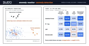
  Isolation Forest (raw)   {'far from usual place': '4/28', '24h burst': '21/21', 'odd basket': '3/21', 'large amount at midnight': '19/19'}
  Isolation Forest (log)   {'far from usual place': '1/28', '24h burst': '21/21', 'odd basket': '12/21', 'large amount at midnight': '8/19'}
  LOF                      {'far from usual place': '1/28', '24h burst': '1/21', 'odd basket': '0/21', 'large amount at midnight': '1/19'}
  Autoencoder              {'far from usual place': '8/28', '24h burst': '21/21', 'odd basket': '0/21', 'large amount at midnight': '15/19'}
With anomalies in the training set, every model misses one type. The raw Isolation Forest catches all of the bursts and the large midnight amounts but only 3/21 odd baskets; the autoencoder catches 0/21 odd baskets (see below for the cause); the log version of Isolation Forest does the opposite, catching 12/21 odd baskets but losing the large amounts. No model catches the "far from usual place" class well either (the best is 8/28), even though a single distance column is enough to see it. That is why combining Isolation Forest (log) and the autoencoder by average rank gives a ROC AUC of 0.973 but an AP of 0.488, which does not beat the best single model: blending models only helps when they are wrong in different places and do not drag each other down.
The autoencoder when training data is normal only
The autoencoder missing the odd baskets entirely may be caused by the training set itself being contaminated: the 211 anomalies skew both the StandardScaler and the loss function. The standard deviation of items is 1.751 with anomalies mixed in and 1.411 when clean. We rerun with the scaler and the network seeing only normal data:
[Autoencoder z=2: scaler and training on normal-only train]
  Autoencoder (clean train)     ROC AUC=1.000 | AP=0.945 | precision@89=0.876
  Autoencoder (clean train) {'far from usual place': '28/28', '24h burst': '21/21', 'odd basket': '21/21', 'large amount at midnight': '8/19'}
AP rises from 0.536 to 0.945 and the odd baskets are caught 21/21, but the large-midnight-amount group drops to 8/19. This supports the contamination hypothesis, but we have not separated the effect of the scaler from that of the network.
Comparing the three anomaly detection approaches
| Criterion | Isolation Forest | LOF | Autoencoder |
|---|---|---|---|
| Time in this article | 1.67 s | 3.90 s | 7.5 s (CPU) |
| Needs scaling/log | Not required; log changes the result (AP 0.590 down to 0.496) because random split thresholds depend on scale | Yes, it relies on distances | Yes, it relies on gradients |
| Sensitive parameters | Number of trees, contamination | n_neighbors larger than the anomaly cluster | Bottleneck size, seed |
| Stability | High (±0.029 AP raw, ±0.032 log) | Depends on clean training data | Low (AP 0.190–0.770) |
| Explaining results | Hard, but SHAP can be used | Hard | Look at per-feature error |
Advice for anomaly detection: start with Isolation Forest because it is fast, stable and has few parameters; treat LOF as a control; use an autoencoder when the data is high-dimensional and structured (sequences, images, logs). Look at the per-feature reconstruction error to explain why a transaction was flagged, in the spirit of Explaining models with SHAP: understanding why a model decides.
When not to use unsupervised anomaly detection
- You already have enough fraud labels: a supervised model such as gradient boosting (see Gradient boosting with XGBoost and LightGBM: when it beats deep learning) usually does better, and the anomaly score can be used as an input feature.
- Anomaly detection flags "legitimate" cases: wholesale buyers or promotion days are also unusual but not fraudulent; you need feedback from the business.
- The distribution drifts over time: retrain periodically and monitor the alert rate.
Common mistakes in anomaly detection
- Trusting
contamination="auto": in this article it flags 15.4% of samples. Choose the threshold according to how many alerts your operations team can handle. - Forgetting to flip the sign of
score_samples: low scores are anomalous, and passing them straight intoroc_auc_scoregives inverted results. - Letting LOF use a small k when the training data contains anomaly clusters: ROC AUC 0.466 versus 1.000 at k = 100.
- Scoring anomaly detection with accuracy: at a 0.5% rate, always guessing "normal" is already 99.5% correct.
- Drawing conclusions from one seed in autoencoder anomaly detection: AP ranges from 0.190 to 0.770.
- A bottleneck that is too wide: the network learns the identity function, AP 0.019 at z = 4.
Checklist
- For anomaly detection, decide clearly between outlier detection (noisy train) and novelty detection (clean train).
- Report ROC AUC, AP and precision@K against the chance level; do not use accuracy.
- Isolation Forest anomaly detection: enough trees (200 or more), try both raw and log versions, set
contaminationfrom the estimated rate. - LOF anomaly detection:
novelty=Trueto score new data, k larger than the smallest anomaly cluster. - Autoencoder anomaly detection: a narrow bottleneck, several seeds, standardized input, inspect the per-feature error.
- Check anomaly detection by anomaly type, and keep a feedback loop from the business to choose the threshold.
The full source is in code/s7-17 (anomaly_demo.py, output.txt, requirements.txt), run with python anomaly_demo.py. Every number is real output from an Apple Silicon machine with 16 GB, CPU, fixed seeds. The anomaly types are generated by us, so this is not an algorithm leaderboard. Original sources: Isolation Forest (Liu, Ting, Zhou, ICDM 2008), Anomaly detection: a survey (Chandola et al., 2009) and Reducing the dimensionality of data with neural networks (Hinton, Salakhutdinov, 2006).
Next article
Sales forecasting with time series: baselines, ARIMA and gradient boosting. When data is ordered in time, every independence assumption in this article no longer holds: the next article builds baselines, ARIMA and gradient boosting with time-aware validation.