On tabular data, meaning tables whose rows are customers, orders or transactions and whose columns are attributes, the model that wins many competitions and runs in many real scoring systems is usually not a neural network. It is gradient boosting on decision trees. This article starts from the core idea (each new tree learns what the previous trees got wrong), builds a gradient boosting model of about 12 lines from scratch, and then compares XGBoost, LightGBM, scikit-learn and a neural network on the same data with real measurements, including the cases where the neural network does not lose.
This article continues Feature engineering for tabular data: encoding, scaling and data leakage; tree models do not need scaling, so much of that work gets lighter here. The evaluation workflow reuses Machine learning with scikit-learn: Pipeline, cross-validation and tuning and the metrics from Model evaluation for classifiers: precision, recall, ROC and imbalanced data.
Environment: Apple M4, 16 GB, no GPU. The APIs used here (early_stopping_rounds in the XGBoost constructor, LightGBM's lgb.early_stopping, HistGradientBoostingRegressor) have been documented since XGBoost 1.6, LightGBM 3.3 and scikit-learn 1.2. A note in the interest of honesty: the numbers in this article come from a run with library versions newer than the publication date (see requirements.txt). We could not rerun on the older versions, so the numbers may differ slightly if you use an older release.
How gradient boosting works
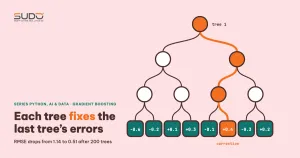
The idea was presented by Jerome Friedman in 2001 in "Greedy Function Approximation: A Gradient Boosting Machine": build a model as a sum F(x) = F0 + η·f1(x) + η·f2(x) + ..., where each f_k is a small tree trained to reduce the loss of the current sum. Concretely, in each round we compute the negative gradient of the loss with respect to the current prediction, then train a new tree to approximate it. With squared loss, the negative gradient is exactly the residual y - F(x), so each tree learns precisely the part the model currently gets wrong. The factor η (the learning rate) shrinks each tree's contribution so that no single tree throws the model off.
The difference from a random forest: a random forest trains many independent trees on different samples and averages them (reducing variance), while gradient boosting trains trees sequentially, each one correcting the errors of the previous ones (reducing bias). That is why gradient boosting is usually more accurate when well tuned, but also overfits more easily if you let it run too long.
We verify this by implementing it ourselves. The data is California Housing, built into scikit-learn (20,640 block groups, 8 features, the label is the median house value in units of $100,000, from the 1990 US census), split 80/20:
class MiniGB:
    def __init__(self, n=200, lr=0.1, depth=3): self.n, self.lr, self.depth = n, lr, depth
    def fit(self, X, y):
        self.f0 = y.mean(); pred = np.full(len(y), self.f0); self.trees = []
        for _ in range(self.n):
            resid = y - pred                         # with squared loss, the negative gradient is exactly the residual
            t = DecisionTreeRegressor(max_depth=self.depth, random_state=0).fit(X, resid)
            pred += self.lr * t.predict(X); self.trees.append(t)
        return self
    def predict(self, X, upto=None):
        p = np.full(len(X), self.f0)
        for t in self.trees[:upto]: p += self.lr * t.predict(X)
        return p
[1] California Housing: (20640, 8) | train 16512 | test 4128 | standard deviation of y: 1.154
[2] Gradient boosting implemented with DecisionTreeRegressor (squared loss, learning_rate=0.1, max_depth=3)
0 trees: RMSE test = 1.1421
1 tree: RMSE test = 1.0841
10 trees: RMSE test = 0.8075
50 trees: RMSE test = 0.5769
200 trees: RMSE test = 0.5053
Compared with sklearn GradientBoostingRegressor, same parameters: RMSE test = 0.5053 | MiniGB = 0.5053With gradient boosting, zero trees (predicting only the mean) give an RMSE of 1.1421, close to the standard deviation of the label; each added tree pulls the error down, and after 200 trees the RMSE is 0.5053. The hand-written version matches to 4 digits the scikit-learn GradientBoostingRegressor with the same parameters, which means the library does nothing more mysterious than the loop above when the loss is squared error.
XGBoost and LightGBM: two implementations of gradient boosting
Both libraries keep the gradient boosting framework above but improve it heavily on the engineering side. The paper XGBoost: A Scalable Tree Boosting System (Chen and Guestrin, KDD 2016) lists three main contributions: a sparsity-aware algorithm, a weighted quantile sketch for finding approximate split points, and a cache-aware design for memory access. Mathematically, the XGBoost documentation describes an objective made of the loss plus a regularization term Ω(f) = γT + ½λΣw², which penalizes the number of leaves T and the magnitude of the leaf scores w. The loss is expanded with a second-order Taylor approximation, so each leaf has an optimal value w* = -G/(H+λ), and a split is kept only if its gain minus γ stays positive, which is the pruning mechanism.
LightGBM, according to the Features documentation, rests on three things. The histogram algorithm groups continuous values into discrete bins, so the cost of finding a split depends on the number of bins rather than the number of rows. Trees grow leaf-wise (best-first): it always splits the leaf with the largest loss reduction, instead of splitting every node at the same depth as level-wise growth does; with the same number of leaves this usually reaches a lower loss, but the documentation warns that it can overfit on small data. And categorical variables are handled directly by sorting the values by sum_gradient / sum_hessian and then searching for the best split along that order, with no one-hot encoding.
One more thing to know: scikit-learn's HistGradientBoostingRegressor (the same histogram family as LightGBM) is an option with no external dependency, which makes it a good starting point when the deployment environment is restricted.
Comparing gradient boosting with other models on the same data
We train gradient boosting and 6 other models on 16,512 training rows and measure RMSE on 4,128 test rows the models have never seen. The neural network (scikit-learn's MLP, two hidden layers of 64 units) has both features and label standardized so the comparison is fair.
  DecisionTree(max_depth=8)          RMSE test = 0.6679 | train 0.05s | predict 0.000s
  RandomForest(300 trees)            RMSE test = 0.5112 | train 3.46s | predict 0.080s
  sklearn GradientBoosting(300)      RMSE test = 0.4669 | train 9.19s | predict 0.013s
  sklearn HistGradientBoosting       RMSE test = 0.4406 | train 9.09s | predict 0.041s
  XGBoost(300, depth=6, lr=0.1)      RMSE test = 0.4430 | train 0.95s | predict 0.004s
  LightGBM(300, leaves=31, lr=0.1)   RMSE test = 0.4387 | train 1.53s | predict 0.013s
  MLP (64-64, X and y standardized)  RMSE test = 0.5766 | train 1.05s | predict 0.002s
Three conclusions about gradient boosting from the table. First, the three histogram-based gradient boosting libraries (HistGradientBoosting, XGBoost, LightGBM) give an RMSE between 0.4387 and 0.4430, less than 1% apart, so choose among them by ecosystem, speed and features rather than accuracy. Second, scikit-learn's classic gradient boosting (not histogram-based) is clearly slower: 9.19 seconds versus 0.95 seconds for XGBoost, and (in this depth=4 configuration) slightly less accurate. Third, the random forest (0.5112) and the single tree (0.6679) clearly lose to boosting on this problem.
Early stopping and learning rate in gradient boosting
The optimal number of trees in gradient boosting is not known in advance. The standard approach is to set n_estimators very high, set a small learning rate, and let the model stop early when the score on a validation set has not improved for a number of rounds. We split off another 20% of the training set as validation (the test set stays untouched):
xg = XGBRegressor(n_estimators=3000, learning_rate=0.05, max_depth=6, tree_method="hist",
                  early_stopping_rounds=30, random_state=0)
xg.fit(X_fit, y_fit, eval_set=[(X_val, y_val)], verbose=False)

lg = LGBMRegressor(n_estimators=3000, learning_rate=0.05, num_leaves=31, random_state=0, verbose=-1)
lg.fit(X_fit, y_fit, eval_set=[(X_val, y_val)], eval_metric="rmse",
       callbacks=[lgb.early_stopping(30, verbose=False)])
XGBoost : best_iteration = 894 / 3000 | RMSE val = 0.4536 | RMSE test = 0.4468
LightGBM: best_iteration = 804 / 3000 | RMSE val = 0.4512 | RMSE test = 0.4467Both stop at roughly 800 to 900 trees out of a maximum of 3,000, and the test RMSE is almost identical (0.4468 and 0.4467). Note that this is not better than the 300-tree model at learning rate 0.1 in the previous table (0.4387 to 0.4430), because this time the model only gets 80% of the training data: early stopping trades some data for safety against overfitting. In practice, people often use early stopping to find the best number of trees and then retrain on all the data with that number of trees.
Overfitting in gradient boosting: num_leaves and leaf-wise trees
The parameter that sets the complexity of LightGBM-style gradient boosting is num_leaves. We increase it with 300 trees and min_child_samples=5 (deliberately loose so the effect is visible):
  num_leaves=4     RMSE train = 0.4857 | RMSE test = 0.5064
  num_leaves=15    RMSE train = 0.3657 | RMSE test = 0.4541
  num_leaves=63    RMSE train = 0.1989 | RMSE test = 0.4336
  num_leaves=255   RMSE train = 0.0453 | RMSE test = 0.4550
  num_leaves=1023  RMSE train = 0.0005 | RMSE test = 0.4981
This is the classic overfitting curve of gradient boosting. The training RMSE keeps falling down to 0.0005 (the model memorizes the data), while the test RMSE falls until num_leaves=63 (0.4336) and then rises again: 0.4550 at 255 leaves and 0.4981 at 1,023 leaves. Tuning is worthwhile, but the gap is small, whereas choosing wrong in the too-complex direction costs more than 0.06 of RMSE.
When gradient boosting beats deep learning, and when it does not
The paper Why do tree-based models still outperform deep learning on tabular data? (Grinsztajn, Oyallon, Varoquaux, 2022) compares methods on 45 tabular datasets and concludes that tree-based models still lead on medium-sized data (about 10,000 samples), even before counting their speed advantage. The authors tie this to differences in inductive bias and name three challenges for neural networks built for tabular data: being robust to uninformative features, preserving the orientation of the data, and learning irregular functions. We test those three ideas on our own data, with a larger MLP (128-128) compared against LightGBM:
     300 train rows: LightGBM RMSE = 0.6768 | MLP RMSE = 0.6709
    1000 train rows: LightGBM RMSE = 0.5642 | MLP RMSE = 0.6344
    5000 train rows: LightGBM RMSE = 0.4935 | MLP RMSE = 0.5648
   16512 train rows: LightGBM RMSE = 0.4680 | MLP RMSE = 0.5113
  MLP (128-128) forgetting to standardize y, 300 rows: RMSE = 7.1466 (versus 0.6709 when y is standardized)

    Adding 20 pure-noise columns (useless features) to the 8 original columns, full 16,512 training rows:
  8 original columns    LightGBM RMSE = 0.4680 | MLP RMSE = 0.5181
  8 original + 20 noise LightGBM RMSE = 0.4768 | MLP RMSE = 0.7358
The most notable finding is about useless features: adding 20 noise columns made LightGBM worse by only 0.009 (0.4680 to 0.4768) but made the MLP worse by 0.218 (0.5181 to 0.7358). Trees ignore columns that do not reduce the loss, while a neural network has to learn zero weights for them. On data size, at 300 rows the two models are even (0.6768 and 0.6709, with the MLP slightly ahead); from 1,000 rows upward LightGBM leads consistently. To be honest: gradient boosting does not always win. With very small data, the result depends on how well each side is tuned, and a single run with a single seed is not enough to be conclusive.
Cases where a neural network makes more sense than gradient boosting: data with structure that trees cannot capture (images, text, audio, long sequences); a need to learn a representation shared across tasks or to combine with embeddings; and very large data that can be trained on a GPU for a long time. For ordinary tables, gradient boosting is still the strongest baseline to try first.
Gradient boosting with categorical variables and missing values
Tree-based gradient boosting handles missing values naturally: XGBoost learns a default direction for missing data at each split node, and LightGBM does something similar. Categorical variables are also supported directly. We generate a synthetic table with a categorical variable of 200 values, two numeric variables and 20% missing values in one column, with label noise of standard deviation 0.5:
  missing rate in num1: 20.2%
  LightGBM, native category column + NaN  : RMSE test = 0.9672
  XGBoost enable_categorical + NaN        : RMSE test = 0.9963
  LightGBM, codes 0..199 as plain numbers : RMSE test = 1.0280
  (the label noise has standard deviation 0.5, so RMSE cannot go much below 0.5; each categorical value has only ~30 training rows)
All three are far from the 0.5 floor because each categorical value has only about 30 training rows, and 20% of the num1 data is missing, so this result should only be read as a relative comparison. Handling the category type properly in LightGBM (0.9672) beats treating the codes 0..199 as plain numbers (1.0280), because trees on plain numbers can only split on an ordinal threshold, which these codes do not have. XGBoost with enable_categorical=True sits in between (0.9963).
Feature importance in a gradient boosting model
XGBoost's gradient boosting model provides importance by gain out of the box (the total loss reduction from the splits that use that feature):
  MedInc     46.2%
  AveOccup   14.7%
  Longitude  11.9%
  Latitude   10.5%
  HouseAge   7.2%
  AveRooms   4.2%
  AveBedrms  2.8%
  Population 2.7%
The block's median income (MedInc) accounts for 46.2% of total gain, which fits real estate experience, and longitude plus latitude (22.4%) together show that geographic location matters. But gain-based importance is a biased measure that favors variables with many possible splits (continuous variables, high-cardinality variables) and does not tell you the direction of the effect. For a more trustworthy explanation, we use SHAP, the topic of the next article in the series.
When not to use gradient boosting
- Unstructured data such as images, text and audio: convolutional neural networks and Transformers are a much better fit.
- Extrapolation beyond the training range (for example forecasting a steadily rising trend): trees predict a constant per leaf, so they do not extrapolate.
- Very tight latency and model size limits: gradient boosting with thousands of trees can be heavier than a small linear model; measure it.
- A need for a simple explanation for end users: logistic regression or a shallow tree is easier to present; gradient boosting needs tools like SHAP.
Common gradient boosting mistakes
- Not using early stopping in gradient boosting, or using the final test set as the validation set, which makes the score optimistic.
- Setting a large learning rate and a few hundred trees and then concluding the model is "optimized"; try a smaller learning rate with early stopping.
- Increasing
num_leaveswithoutmin_child_samples, which leads to trees that memorize the data, as in the num_leaves=1023 row of the table. - Encoding categorical variables as ordinal numbers and treating them as plain numbers, when the library supports the
categorytype. - Comparing against a neural network while forgetting to standardize the label; our first run forgot this and gave the MLP (128-128, only X standardized, y not standardized) an RMSE of 7.1466 on 300 training rows, more than ten times the 0.6709 obtained when y is standardized (the last line of section [6] in
gb_demo.pyreproduces this number), a wrong conclusion caused by a preparation error and not by the model.
Gradient boosting checklist
- Start with gradient boosting (
HistGradientBoosting, LightGBM or XGBoost defaults) as a strong baseline before thinking about neural networks. - With gradient boosting, use a small learning rate (0.03 to 0.1), a large
n_estimatorsand early stopping on a separate validation set. - Tune gradient boosting through
num_leaves/max_depthandmin_child_samples; watch the gap between training and test RMSE. - Use the
categorytype and missing values directly, and do not one-hot encode high-cardinality variables. - Compare against a simple model and a neural network on the same test set with the same preparation workflow.
- Touch the test set once; pin library versions (for example with
requirements.txt), because defaults and measurements can change between releases.
The full source code is in code/s7-14 (gb_demo.py, output.txt, requirements.txt). On macOS, LightGBM needs the OpenMP library: if it is missing, install libomp with Homebrew or point DYLD_FALLBACK_LIBRARY_PATH to the libomp.dylib that ships with scikit-learn. All numbers are real output from an Apple M4, 16 GB; the timings come from a single run and are not a rigorous benchmark.
Next article
Explaining models with SHAP: understanding why a model decides. A gradient boosting model is accurate but a black box; the next article uses Shapley values to explain each prediction and compares them with traditional feature importance.