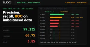
A fraud-detection model with 99.13% accuracy sounds impressive, until you learn that a program that prints "not fraud" for every transaction scores 99.12%. That is why model evaluation for classifiers cannot stop at a single accuracy number, especially on imbalanced data, where one class is far rarer than the other: fraud, rare diseases, customer churn. This article walks through the confusion matrix, precision, recall, F1, ROC AUC, average precision, cost-based threshold selection and class_weight. Every concept comes with real output from a simulated set of 20,000 transactions in which only 0.88% are positive.
This model evaluation guide follows Machine learning with scikit-learn: Pipeline, cross-validation and tuning, where we used roc_auc and f1 without explaining them, and Linear regression and gradient descent: implementing it with NumPy. For the overall workflow, see What is machine learning: problems, data and the workflow of an AI project. Environment for rerunning: Apple M4, 16 GB, Python 3.10, scikit-learn 1.2.0 (released December 2022), NumPy 1.23.5. The data is entirely simulated.
The confusion matrix: the foundation of model evaluation
In a binary problem, every prediction falls into one of four cells: true positive (tp, predicted positive and correct), false positive (fp, predicted positive but wrong), false negative (fn, a miss) and true negative (tn). According to the scikit-learn Metrics and scoring documentation, confusion_matrix has true classes in rows and predicted classes in columns, so cell (i, j) counts observations that truly belong to class i but were predicted as class j. For a binary problem you can get the four numbers with tn, fp, fn, tp = confusion_matrix(y_true, y_pred).ravel().
| Metric | Formula | The question it answers |
|---|---|---|
| Accuracy | (tp + tn) / total | Share of correct predictions, regardless of class |
| Precision | tp / (tp + fp) | Of the transactions flagged as fraud, how many are really fraud? |
| Recall (sensitivity) | tp / (tp + fn) | Of the real fraud cases, how many did we catch? |
| F1 | 2·P·R / (P + R) | Harmonic mean of precision and recall |
| Balanced accuracy | mean of per-class recall | Accuracy weighted by the inverse of class frequency |
The documentation describes them intuitively: precision is the ability of the classifier not to label a negative sample as positive, and recall is the ability to find all the positive samples. The two metrics pull in opposite directions, so any serious model evaluation must look at both.
Model evaluation on imbalanced data: how accuracy misleads
We generate 20,000 transactions with 8 features. The positive label (fraud) is built from a combination of a few features plus noise, using the 99th percentile as the cutoff. We split 70/30 with stratify=y to keep the class ratio in both parts.
scikit-learn 1.2.0
n = 20000 | positives: 176 | positive rate: 0.88%
test: 6000 samples, positives: 53
The test set has only 53 positives: remember this number, because it limits the reliability of every metric below. In model evaluation, the first baseline in any classification project should be DummyClassifier, the thing a real model has to beat:
dummy = DummyClassifier(strategy="most_frequent").fit(X_tr, y_tr)[Baseline: always predict 'not fraud']
accuracy = 0.9912
recall = 0.0000
balanced_accuracy = 0.5000
roc_auc = 0.5000Accuracy is 0.9912 and recall is 0: the baseline catches no fraud at all, yet it is "right" 99.12% of the time because 99.12% of transactions are normal. Balanced accuracy (0.5) and ROC AUC (0.5) both correctly show that this model is no better than random guessing. According to the scikit-learn documentation, balanced accuracy is designed to avoid inflated scores on imbalanced data: it is the mean of the recall of each class.
Evaluating a real model: logistic regression
We train a logistic regression with StandardScaler in a Pipeline and evaluate it at the default threshold. The predict method of logistic regression assigns the positive class when the probability exceeds 0.5, while the precision_recall_curve documentation shows that precision and recall change with the decision threshold. So 0.5 is just one operating point among countless possible ones, and there is no reason it would be optimal for your business.
[Logistic regression, threshold 0.5]
  confusion matrix (rows=actual, columns=predicted):
 [[5946    1]
 [  51    2]]
  tn=5946 fp=1 fn=51 tp=2
  accuracy  = 0.9913
  precision = 0.6667  (tp/(tp+fp) = 2/3)
  recall    = 0.0377  (tp/(tp+fn) = 2/53)
  F1        = 0.0714
  balanced_accuracy = 0.5188 | MCC = 0.1572
  ROC AUC = 0.9606 | Average precision (PR AUC) = 0.3416 | AP of random guessing = 0.0088
This is a typical picture of model evaluation on imbalanced data. Accuracy of 0.9913 beats the baseline by only 0.0001. The model is right on 2 out of 3 fraud alerts (precision 0.667) but misses 51 of 53 fraud cases (recall 0.038). Meanwhile ROC AUC reaches 0.9606: the model ranks very well, since fraudulent transactions usually score higher than normal ones, but the 0.5 threshold is set so high that it almost never raises an alert. The problem is not the model but the decision threshold. Model evaluation needs both views: ranking metrics (ROC AUC, average precision) and metrics at a specific threshold (precision, recall, F1).
Per-class model evaluation report
              precision    recall  f1-score   support

      normal      0.991     1.000     0.996      5947
       fraud      0.667     0.038     0.071        53

    accuracy                          0.991      6000
   macro avg      0.829     0.519     0.534      6000
weighted avg      0.989     0.991     0.987      6000
classification_report makes it clear: weighted avg (0.987) is dominated by the majority class, while macro avg (0.534) is a simple average across classes and so reflects the rare class. With imbalanced data, when you evaluate a model, read the row of the rare class and the macro avg, not accuracy or weighted avg. matthews_corrcoef (MCC, 0.157 here) is high only when all four cells of the confusion matrix are good.
The decision threshold in model evaluation: trading precision for recall
A model returns only probabilities; the label is the result of comparing the probability with a threshold, and we can choose a different threshold to move to a different operating point. Lowering the threshold catches more fraud (recall goes up) but also raises more false alarms (precision goes down):
[Changing the decision threshold]
 threshold  precision   recall      F1   tp    fp   fn
    0.5      0.667    0.038   0.071    2     1   51
    0.3      0.733    0.208   0.324   11     4   42
    0.2      0.485    0.302   0.372   16    17   37
    0.1      0.287    0.509   0.367   27    67   26
    0.05      0.176    0.679   0.279   36   169   17
The table shows the trade-off when evaluating a model with real numbers: at threshold 0.05, we catch 36 of 53 cases (recall 0.679) but have to review 169 more false alarms (precision 0.176). F1 peaks (0.372) around threshold 0.2, but F1 treats precision and recall as equally important, which is rarely true in a real business.
Choosing a threshold by business cost
The right question is not "which threshold has the highest F1" but "which mistake is more expensive". Suppose missing a fraud case costs 50 units (refunds, reputation), while one unnecessary manual review costs 1 unit. We sweep the threshold and pick the one with the lowest total cost:
Cost: miss=50.0, false alarm=1.0
  threshold 0.5   : cost = 2551
  threshold 0.04  : cost = 918 (tp=39, fp=218, fn=14, recall=0.736, precision=0.152)
  Note: this threshold is chosen on the test set for illustration only; in practice it must be chosen on validation/CV.
Cost-based model evaluation: the cost drops from 2,551 to 918 (about 64%) just by changing the threshold, not the model.
Two important caveats. First, the cost figures 50 and 1 are illustrative assumptions; take them from your real business. Second, in this example we pick the threshold directly on the test set, which violates the rule of touching the test set only once, as covered in the article on Pipeline and cross-validation; in practice you must choose the threshold on validation data or with cross-validation. The right way is to get out-of-sample probabilities with cross_val_predict(..., method="predict_proba") on the training set, sweep the threshold over those probabilities, fix the threshold, and only then apply it to the test set.
Model evaluation with ROC and precision-recall: two different stories
The ROC curve plots the true positive rate (which is recall) against the false positive rate as the threshold varies; ROC AUC summarizes it in one number, and the documentation stresses that it takes probabilities or scores that have not been thresholded, so no threshold has to be chosen. ROC AUC means the probability that a random positive sample gets a higher score than a random negative sample. The precision-recall (PR) curve plots precision against recall, and average_precision_score summarizes it as a weighted sum; according to the documentation, for random predictions AP equals the share of positive samples, which makes it the right reference point.
The big difference appears when the data is imbalanced. Negatives are so numerous that the false positive rate (fp divided by total negatives) stays small even when the absolute fp is large, which makes ROC look good. Precision is not diluted that way. The study by Saito and Rehmsmeier (PLOS ONE, 2015) recommends precision-recall plots over ROC for evaluating binary classifiers on imbalanced data. To check this yourself in model evaluation, we keep the model and all the positives in the test set the same, and only drop or keep negatives to change the positive rate:
[ROC AUC barely changes as the positive rate drops, PR AUC falls sharply]
 positive rate   ROC AUC      AP  AP random
      0.2000     0.956   0.849         0.2000
      0.0500     0.959   0.640         0.0500
      0.0200     0.960   0.470         0.0200
      0.0100     0.961   0.366         0.0100
ROC AUC stays at 0.956 to 0.961 while average precision falls from 0.849 to 0.366, just because the positive class gets rarer. The model did not get worse; the "needle in a haystack" problem got harder, and only PR reflects that. How to read them: ROC AUC answers "how well does the model rank", while AP answers "how clean is my alert list at a given recall". For alerting problems where reviewers have limited capacity, AP matters more in model evaluation.
Handling imbalanced data: class_weight and its effect on model evaluation
The cheapest way to make a model care about the rare class is to set class_weight="balanced", which increases the error weight on the positive class in inverse proportion to its frequency. Compare the two models at threshold 0.5:
[class_weight='balanced' (threshold 0.5)]
  unweighted      precision=0.667 recall=0.038 F1=0.071 ROC AUC=0.961 AP=0.342
  balanced        precision=0.061 recall=0.943 F1=0.115 ROC AUC=0.961 AP=0.356
ROC AUC stays at 0.961 and AP barely changes (0.342 versus 0.356). What class_weight mainly changes is the operating point: recall jumps from 0.038 to 0.943, and in exchange precision falls from 0.667 to 0.061. class_weight is roughly equivalent to shifting the decision threshold, but it skews the output probabilities (they are no longer calibrated). If you need trustworthy probabilities to compute expected cost, keep the original model and tune the threshold, or recalibrate the probabilities.
For model evaluation with resampling, techniques (oversampling, undersampling) are outside core scikit-learn and usually come from the imbalanced-learn library; if you use them, put them inside a Pipeline so they apply only to the training part of each fold. Otherwise they leak data, following the same principle as in the article on Pipeline and cross-validation.
Model evaluation with cross-validation and confidence intervals
A single number on a test set with only 53 positives is very unstable. We use stratified cross-validation with several metrics on the training set to compare two models, logistic regression and random forest:
[Stratified 5-fold CV on the train set]
  LogReg        roc_auc=0.945±0.012 | average_precision=0.239±0.046 | f1=0.151±0.046
  RandomForest  roc_auc=0.918±0.032 | average_precision=0.203±0.054 | f1=0.015±0.030
Logistic regression is slightly ahead on every metric, but it must be read together with the standard deviation: for average precision, 0.239 ± 0.046 versus 0.203 ± 0.054 is a difference within the noise. Note also that the CV AP score (0.239) is much lower than the test set score (0.342): with only a few dozen positives, results change a lot from split to split. The random forest F1 (0.015) in this model evaluation is low because at threshold 0.5 it almost never predicts positive: when retrained on the whole train set, it predicts 0 positives on the 6,000 test samples (output right below), but that does not mean it ranks badly; this is why you should not compare models with threshold-dependent metrics before tuning the threshold.
[Random forest, threshold 0.5, test set] predicted positives = 0 / 6000 (actual positives: 53), recall = 0.000To measure uncertainty directly on the test set, use the bootstrap: resample the test set with replacement 1,000 times and recompute recall:
[Bootstrap 1000 times] test recall = 0.038, 95% confidence interval: [0.000, 0.094] (only 53 positives)In this model evaluation, the wide 95% confidence interval that touches 0 shows large uncertainty. With only 53 positives, every metric of the positive class fluctuates strongly. When evaluating a model, report the interval too, and collect more positive samples before comparing models that are close.
A recommended workflow for classification model evaluation
- Define the business cost of fp and fn before evaluating the model.
- Set a baseline with
DummyClassifierand compare every model evaluation result against it. - Choose the primary metric for the problem: for imbalanced data where the rare class matters, use average precision and recall at an acceptable precision; for balanced data, ROC AUC and accuracy are still reasonable.
- Evaluate with stratified cross-validation and report the mean and standard deviation.
- Tune the threshold on validation data by cost, instead of using the default 0.5.
- Touch the test set once and report it with a confidence interval.
- Monitor after deployment: recompute the metrics periodically, because class ratios and feature distributions change over time.
When common model evaluation metrics are not enough
- Multiple classes: in model evaluation,
average="macro"treats all classes equally,"weighted"follows frequency; state the choice in your report. - Top-k ranking: in model evaluation, if the review team can only handle 100 cases a day, precision@100 is more useful than any AUC.
- Probabilities must be trustworthy (risk pricing, expected cost): you also need calibration metrics such as the Brier score and calibration curves, because AUC does not measure whether the probabilities are correct.
- Data that shifts over time or across groups: split by time or group and evaluate each customer segment separately.
Common mistakes in model evaluation
- Evaluating a model with accuracy alone on imbalanced data: a useless baseline also reaches 99.12% in the example above.
- Using the default 0.5 threshold and concluding the model is bad when recall is low: the model may rank well (ROC AUC 0.96) and only the threshold is wrong.
- Choosing the threshold on the test set: this leaks information; choose it on validation data or use cross-validation.
- Trusting ROC AUC when the positive class is very rare: it barely changes while AP drops sharply.
- Comparing models in model evaluation by differences smaller than the standard deviation, or on too few positives.
- Mixing up argument order: metric functions take
(y_true, y_pred)in that order; swapping them exchanges precision and recall without any error. For ROC AUC and AP, pass the positive-class probability (predict_proba(X)[:, 1]), not thresholded labels. - Forgetting
stratifywhen splitting imbalanced data: the test set may end up with no positives at all.
Model evaluation checklist
- When evaluating a model, always look at the confusion matrix, not just one number.
- Compare with
DummyClassifier; on imbalanced data, use balanced accuracy, recall, precision and average precision. - Read ROC AUC as ranking quality and AP as the quality of the alert list.
- Choose the threshold by business cost on validation data or on probabilities from
cross_val_predict. class_weightmainly shifts the operating point; output probabilities are no longer calibrated.- Report model evaluation results with mean ± standard deviation or a confidence interval, and state the number of positives.
The full source code is in code/s7-12 (eval_demo.py, output.txt, requirements.txt), run with python eval_demo.py. All model evaluation numbers in this article are real output from an Apple M4, 16 GB, scikit-learn 1.2.0, NumPy 1.23.5 with a fixed seed; the data is simulated, and the cost coefficients 50 and 1 are illustrative assumptions.
Next article
Feature engineering for tabular data: encoding, scaling and data leakage. The next step is to improve what we measure: transform features correctly, avoid leakage, and verify the result with the metrics from this article.