Many machine learning projects fail not because the algorithm is weak, but because the team picked the wrong problem, trained on unrepresentative data, or measured results with the wrong yardstick. This article opens the machine learning part of the series: what machine learning is, how it differs from conventional programming, the main problem types, why you must split data into train and test sets, and what steps a project goes through. We go beyond definitions and build a small project that really runs with scikit-learn 1.1.2 on Python 3.10 (Apple M4, 16 GB): predicting whether a customer will buy again within 90 days, comparing against a baseline, and seeing overfitting and data leakage with our own eyes. The data is synthetic, generated with a fixed seed, not real customers.
The article uses tools from the previous two articles in the series: the clean table from Cleaning crawled data with pandas: normalization, deduplication and data types, and arrays, shapes and broadcasting from NumPy for machine learning: vectorization and broadcasting. The input data of many real projects starts with a crawl, so see also Crawling data with Python: requests, BeautifulSoup and robots.txt.
What is machine learning, and how does it differ from conventional programming
In conventional programming, you write rules and feed data through them to get results: if an order is over 2 million and the customer is new, flag it for review. In machine learning, you feed in data together with the known answers, and the algorithm infers the rules from them. The learned rules, called a model, are then applied to new data. This view helps you decide when to use machine learning: when there are too many rules, they are too vague, or they change too often to write by hand, but you have plenty of labeled examples.
It is also worth being modest about where machine learning fits. Google's Rules of Machine Learning opens with its first rule: don't be afraid to launch a product without machine learning. A simple heuristic, such as ranking by install count or filtering publishers that have sent spam before, often takes a product most of the way. Use machine learning only when the product truly needs it and you have data.
Types of machine learning problems
According to the scikit-learn introductory tutorial, data is always represented as a table of shape (n_samples, n_features): each row is a sample and each column is a feature. There are two big groups, distinguished by whether the data comes with answers:
| Group | Problem | Output | Business example |
|---|---|---|---|
| Supervised learning | Classification | discrete label | whether an order is fraudulent; whether a customer returns |
| Supervised learning | Regression | continuous number | next week's sales forecast; house prices |
| Unsupervised learning | Clustering | groups of similar samples | splitting customers into behavior segments |
| Unsupervised learning | Dimensionality reduction, density estimation | a more compact representation, outlier detection | data visualization, detecting unusual transactions |
Most of a company's first machine learning problems are supervised, because historical data already has the answers: whether the customer came back, whether the order was refunded. The first job in a machine learning project is to turn a vague request ("retain customers") into a concrete prediction question ("will customer A buy again in the next 90 days?"), together with the decision that prediction serves (which group gets a voucher).
The machine learning project workflow: six steps
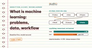
A machine learning project usually follows CRISP-DM, the standard process of the data mining industry, described in the CRISP-DM 1.0 Step-by-step data mining guide (Chapman et al., 2000) with six phases. The phases are not linear: results in a later phase often force you back to an earlier one.
- Business understanding: the goal, the success metric, and the cost of being wrong. This is the phase most often skipped.
- Data understanding: what the data contains, what is missing, how good it is, where the labels come from and whether they can be trusted.
- Data preparation for machine learning: cleaning, feature engineering, and the train and test split. It usually takes most of the project time; pandas and NumPy from the previous two articles belong to this phase.
- Modeling in machine learning: choosing an algorithm, training, and tuning parameters.
- Evaluation: measure on unseen data, compare with the baseline, and check against the business goal, not only against a technical number.
- Deployment and monitoring: put it into a real system and track its performance over time.
The rest of the article covers phases 2 to 5 with code; deployment and monitoring will get their own article.
Building the data and splitting train and test in a machine learning project
The sample project: an online store wants to know which customers will buy again in the next 90 days so it can send offers to the right people. The features are the number of past orders, the number of days since the last order, the average order value, and whether the customer has ever used a voucher; the label quay_lai (returned) is 1 if the customer bought again. Since we do not use real customer data, we generate 3,000 synthetic customers with an assumed relationship between features and label.
# --- 1. Data: 3000 customers, label quay_lai = 1 if they bought again within 90 days ---
rng = np.random.default_rng(7)
n = 3000
so_don = rng.poisson(3, n) + 1
ngay_tu_don_cuoi = rng.integers(1, 365, n)
gia_tri_tb = rng.normal(900_000, 300_000, n).clip(50_000)
da_dung_voucher = rng.integers(0, 2, n)
logit = 0.55 * (so_don - 4) - 0.012 * (ngay_tu_don_cuoi - 120) + 0.0000004 * (gia_tri_tb - 900_000) + 0.4 * da_dung_voucher - 0.6
p = 1 / (1 + np.exp(-logit))
quay_lai = (rng.random(n) < p).astype(int)
df = pd.DataFrame({"so_don": so_don, "ngay_tu_don_cuoi": ngay_tu_don_cuoi,
                   "gia_tri_tb": gia_tri_tb.round(-3), "da_dung_voucher": da_dung_voucher,
                   "quay_lai": quay_lai})
print(df.head(3).to_string(index=False))
print("\nReturn rate:", round(df["quay_lai"].mean(), 3), "| samples:", len(df))

X = df.drop(columns="quay_lai"); y = df["quay_lai"]
X_tr, X_te, y_tr, y_te = train_test_split(X, y, test_size=0.25, random_state=42, stratify=y)
print("train:", len(X_tr), "| test:", len(X_te))
so_don ngay_tu_don_cuoi gia_tri_tb da_dung_voucher quay_lai
5 136 733000.0 0 1
2 364 1197000.0 1 0
5 276 946000.0 0 0
Return rate: 0.294 | samples: 3000
train: 2250 | test: 750About 29% of customers return: the set is imbalanced (class 1 is smaller than class 0). This matters at the evaluation step. We split the data into two parts: a training set (train) from which the model learns, and a test set kept aside to measure how well it generalizes. The scikit-learn documentation defines it exactly this way: the train set is the data from which the model learns its properties, and the test set is data held out to check what was learned. The stratify=y parameter keeps the class ratio equal in both parts, and a fixed random_state makes reruns give the same result.
The vital rule of machine learning: touch the test set only once, at the end. Any choice (features, parameters, algorithm) made based on the test set makes it stop representing unseen data.
Note: in this article we print the test scores of several models back to back purely for illustration, because the goal is to show what a baseline and overfitting look like. In a real project, choose the model and parameters (such as max_depth) with cross-validation on the train set, as in the later section, and only then measure the test set exactly once for the chosen model. The full code (including the import lines) for the snippets below is in the article's two files, project.py and leakage.py.
Baseline first, machine learning model second
Before training anything, establish the simplest point of comparison. For classification, that is always guessing the majority class (DummyClassifier). A machine learning model is only worth something if it clearly beats the baseline. We compare the baseline with logistic regression (placed after a StandardScaler scaling step in a Pipeline) and print accuracy, precision and recall on both train and test:
def report(name, model):
    model.fit(X_tr, y_tr)
    for tag, Xs, ys in (("train", X_tr, y_tr), ("test ", X_te, y_te)):
        pr = model.predict(Xs)
        print(f"{name:<22} {tag} acc={accuracy_score(ys, pr):.3f} "
              f"precision={precision_score(ys, pr, zero_division=0):.3f} recall={recall_score(ys, pr):.3f}")

# --- 2. Baseline first, model second ---
print("\n=== Baseline and model ===")
report("Baseline (majority)", DummyClassifier(strategy="most_frequent"))
report("Logistic regression", make_pipeline(StandardScaler(), LogisticRegression(max_iter=1000)))
=== Baseline and model ===
Baseline (majority) train acc=0.706 precision=0.000 recall=0.000
Baseline (majority) test acc=0.705 precision=0.000 recall=0.000
Logistic regression train acc=0.783 precision=0.680 recall=0.495
Logistic regression test acc=0.795 precision=0.725 recall=0.489The baseline uses no machine learning and still reaches an accuracy of 0.705 without learning anything, simply because 70% of customers do not return. But its recall is 0: it finds no customer who will return, which makes it useless for the goal of sending offers. This shows why accuracy alone is misleading on imbalanced data. Logistic regression reaches an accuracy of 0.795 on test, about 9 percentage points above the baseline, and finds about 49% of the customers who actually return, with a precision of 0.725.
A machine learning model that is modest but genuinely useful; precision and recall will be covered in detail in a separate article on model evaluation. For now, understand that precision is the share of "will return" predictions that are actually right, and recall is the share of truly returning customers that the model manages to find.
Overfitting: memorizing is not learning
Overfitting happens when a model fits the training data too closely, in effect memorizing the noise as well, and then predicts poorly on new data. The scikit-learn cross-validation documentation calls learning the parameters and testing on the same data a methodological mistake: a model that simply repeats the labels it has just seen would get a perfect score but fail to predict anything useful on new data. A decision tree with no depth limit is the classic example, because it can keep splitting until every leaf holds a single sample:
# --- 3. Overfitting: a tree with no depth limit ---
print("\n=== Overfitting ===")
report("Unlimited-depth tree", DecisionTreeClassifier(random_state=0))
report("Limited tree (depth=3)", DecisionTreeClassifier(max_depth=3, random_state=0))
=== Overfitting ===
Unlimited-depth tree train acc=1.000 precision=1.000 recall=1.000
Unlimited-depth tree test acc=0.680 precision=0.455 recall=0.430
Limited tree (depth=3) train acc=0.780 precision=0.688 recall=0.462
Limited tree (depth=3) test acc=0.752 precision=0.634 recall=0.376The unlimited-depth tree reaches an accuracy of 1.000 on train but only 0.680 on test, even lower than the 0.705 baseline. The 0.32 gap between the two numbers is the signature of overfitting. Limiting max_depth=3 forces the tree to learn more general patterns: train 0.780, test 0.752, a gap of only 0.028. The takeaway: accuracy on the training set says nothing about real quality; only the gap between train and test tells you whether the model generalizes. Ways to fight overfitting: add more data, reduce model complexity, and evaluate properly.
Cross-validation: a more stable evaluation than a single split
A single train and test split gives a number that depends on the luck of which samples land where. Cross-validation splits the train set into 5 folds, holds out one fold at a time for validation, trains on the other four, then takes the mean and standard deviation. It is used to compare models and choose parameters without touching the test set:
# --- 4. A more stable evaluation: 5-fold cross-validation on the train set ---
print("\n=== Cross-validation (5 folds, train set) ===")
for name, m in (("Logistic regression", make_pipeline(StandardScaler(), LogisticRegression(max_iter=1000))),
                ("Tree depth=3", DecisionTreeClassifier(max_depth=3, random_state=0))):
    s = cross_val_score(m, X_tr, y_tr, cv=5, scoring="accuracy")
    print(f"{name:<22} acc = {s.mean():.3f} ± {s.std():.3f}")
=== Cross-validation (5 folds, train set) ===
Logistic regression acc = 0.784 ± 0.018
Tree depth=3 acc = 0.773 ± 0.009Logistic regression reaches 0.784 ± 0.018 and the depth-3 tree reaches 0.773 ± 0.009. The two models are close within the range of variation, so the 0.011 difference is not enough to conclude which model is better. That is why you need to look at the standard deviation, not just the mean.
Data leakage: when a result is suspiciously good
The most dangerous mistake in a machine learning project is data leakage. Data leakage is using information that will not be available at real prediction time to build the model, so the performance estimate becomes overly optimistic and the model does worse in production. Common causes include mixing train with test, calling fit on test data, and learning preprocessing parameters (such as the mean used for scaling) from the entire dataset.
On that last principle, the scikit-learn 1.1 documentation is explicit: preprocessing steps such as scaling or feature selection must also be learned from the training set and only then applied to held-out data, and Pipeline helps do exactly that during cross-validation. The way to avoid leakage is to split the data before any preprocessing step and use a Pipeline so each step learns only from the train part of each split.
There is a subtler form of leakage: a feature that carries information from the future. For example, adding a column "orders in the next 90 days" to the problem of predicting the next 90 days. This column cannot exist at prediction time, yet in the historical table it is sitting right there. See how it changes the result:
rng = np.random.default_rng(7)
n = 3000
X = pd.DataFrame({"so_don": rng.poisson(3, n) + 1, "ngay_tu_don_cuoi": rng.integers(1, 365, n)})
logit = 0.55 * (X["so_don"] - 4) - 0.012 * (X["ngay_tu_don_cuoi"] - 120) - 0.2
y = (rng.random(n) < 1 / (1 + np.exp(-logit))).astype(int)

def cv(Xs):
    m = make_pipeline(StandardScaler(), LogisticRegression(max_iter=1000))
    return cross_val_score(m, Xs, y, cv=5).mean()

print(f"Valid features     : acc = {cv(X):.3f}")
X_leak = X.assign(don_trong_90_ngay_toi=y + rng.integers(0, 2, n) * y)   # only known AFTER the prediction time
print(f"With leaky feature : acc = {cv(X_leak):.3f}  <- suspiciously good")
Valid features : acc = 0.780
With leaky feature : acc = 1.000 <- suspiciously goodWith valid features, cross-validation gives 0.780. Add the leaky feature and accuracy jumps to 1.000, a perfect result that almost never happens in reality. A result that is too good is a sign to be suspicious before celebrating. For every feature, ask yourself: at the moment the system needs to predict, does this value exist yet?
When not to use machine learning
- Clear and stable rules: tax calculation, tiered discounts, format validation. Writing the rules directly is more accurate and easier to verify.
- Not enough labeled data: with machine learning, a few dozen samples are not enough to learn a reliable pattern; wrong labels are even worse than missing labels.
- Errors with severe consequences that need explanation: credit or medical decisions require explainability and their own control processes.
- A heuristic is already good enough: following Google's rule above, start with a heuristic and add machine learning only when there is evidence that it improves things.
- Training data does not look like real data: a model that learns from the past is valid only as long as the future resembles the past.
Common mistakes in machine learning projects
- Skipping the baseline: you do not know whether the machine learning model beats guessing the majority class.
- Looking only at accuracy of a machine learning model on imbalanced data; always check precision and recall as well.
- Tuning on the test set in machine learning: choosing parameters by test score and then reporting that same score; use cross-validation on the train set instead.
- Scaling before splitting: computing the mean and standard deviation on the whole dataset is a form of leakage; put
StandardScalerinside aPipeline. - Features from the future: check that every column exists at prediction time.
- Forgetting the deployment path: Google advises getting the whole system running end to end with a simple model first, and only then upgrading it.
- Confusing correlation with causation: a machine learning model seeing that customers who use vouchers tend to return does not mean handing out vouchers will make them return.
Checklist for starting a machine learning project
- For every machine learning project, write the problem as one concrete prediction sentence, with the decision the prediction serves and the cost of being wrong.
- Identify where the label comes from and the prediction time, so you can check that no feature comes from the future.
- Split train and test before any preprocessing step; fix
random_state; usestratifywhen classes are imbalanced. - Set a simple baseline; the model must beat the baseline on a metric that reflects the business goal.
- Compare models with cross-validation on the train set; compare the train and test gap to detect overfitting.
- Read an overly good result as a warning; touch the test set once at the end.
- Record library versions, seeds and data so the results can be reproduced.
In short, machine learning is a way for a machine to infer rules from data with answers, and its quality depends more on a correctly posed problem, representative data and honest evaluation than on a fancy algorithm. With a six-step process, a baseline and discipline in splitting data, you have avoided most of the common failures.
Next article
This article used a linear model without explaining how it learns. The next article implements that part from scratch: the loss function, the derivative and the parameter update loop in NumPy. Continue with Linear regression and gradient descent: implementing it with NumPy.