Almost every modern machine learning model, from linear regression to neural networks with billions of parameters, is trained with the same idea: measure the error, compute the slope, take a small step against the slope, and repeat. That idea is gradient descent. This article implements gradient descent from scratch in NumPy for a linear regression problem (predicting room rent), verifies the gradient with finite differences, runs it for real, and compares the result with the closed-form solution and scikit-learn's LinearRegression. You will see for yourself why the learning rate decides between convergence and divergence, and why feature scaling is not a "trick" but a condition for the algorithm to run stably.
This article builds on NumPy for machine learning: vectorization and broadcasting (every loop below is vectorized) and fits into the workflow described in What is machine learning: problems, data and the workflow of an AI project. Environment: Apple M4, 16 GB, Python 3.10, NumPy 1.23.1, scikit-learn 1.1.2 (used only for the final comparison), the same versions as the two previous articles in the series. The code uses only basic NumPy operations (default_rng has existed since NumPy 1.17), so it runs on older releases too.
The problem: what linear regression is
Linear regression predicts a real number from features using a linear combination: y_hat = b + w1*x1 + w2*x2 + .... For a feature matrix X of shape (n samples, p features), we add a column of ones so that b becomes part of the parameter vector theta; the prediction is then X @ theta. The goal is to choose theta so that the sum of squared errors is as small as possible. The scikit-learn documentation on Ordinary Least Squares describes exactly this: the model minimizes the residual sum of squares between the observed and the predicted values.
The loss function we use is the mean squared error:
L(theta) = (1/n) * sum( (X @ theta - y)^2 )
dL/dtheta = (2/n) * X.T @ (X @ theta - y)
The second formula is the gradient: the vector pointing in the direction in which the loss increases fastest. Gradient descent walks the opposite way: theta = theta - lr * gradient, where lr is the learning rate (step size). The loss of linear regression is a convex function (a single "bowl"), so gradient descent with a small enough lr always reaches the same bottom as the closed-form solution. That makes it an ideal exercise for checking your own implementation.
Synthetic data: room rent
We generate data with a known answer so we can compare: rent (million VND per month) = 1.2 + 0.11 × area (m²) − 0.25 × distance to the center (km) + noise. The data is entirely synthetic and does not belong to anyone.
import numpy as np

rng = np.random.default_rng(42)
n = 200
dien_tich = rng.uniform(15, 60, n)         # area in m²
khoang_cach = rng.uniform(0.5, 12, n)      # distance to center in km
nhieu = rng.normal(0, 0.4, n)              # noise
y = 1.2 + 0.11 * dien_tich - 0.25 * khoang_cach + nhieu
X = np.column_stack([dien_tich, khoang_cach])
Xb = np.column_stack([np.ones(n), X])      # add the bias column
The closed-form solution as a baseline
Before iterating, get the reference answer with least squares. Do not invert X.T @ X yourself; use np.linalg.lstsq, which solves the problem with a more numerically stable decomposition. scikit-learn also computes its solution with the singular value decomposition of X, at a cost of about O(n_samples × n_features²) according to its documentation.
theta_ls, *_ = np.linalg.lstsq(Xb, y, rcond=None)
print("[lstsq] theta =", np.round(theta_ls, 4))
[lstsq] theta = [ 1.0692 0.1136 -0.2538]The result does not match 1.2 / 0.11 / −0.25 exactly because of the noise and the small sample of 200 rows. It is the optimal solution for this dataset, and it is the target that gradient descent must reach.
Implementing gradient descent step by step
Two functions are enough for the whole gradient descent algorithm: the loss and the gradient, each a single vectorized NumPy line. The main loop updates theta, records the loss history, and stops when the loss barely changes or when it detects divergence.
def mse(theta, Xb, y):
    r = Xb @ theta - y
    return float(r @ r / len(y))

def grad(theta, Xb, y):
    r = Xb @ theta - y
    return 2.0 / len(y) * (Xb.T @ r)

def gradient_descent(Xb, y, lr, n_iter, tol=1e-10):
    theta = np.zeros(Xb.shape[1])
    hist = [mse(theta, Xb, y)]
    for i in range(n_iter):
        theta = theta - lr * grad(theta, Xb, y)
        hist.append(mse(theta, Xb, y))
        if not np.isfinite(hist[-1]) or hist[-1] > 1e12:
            return theta, hist, i + 1, "diverged"
        if abs(hist[-2] - hist[-1]) < tol:
            return theta, hist, i + 1, "converged"
    return theta, hist, n_iter, "max iterations"
Checking the gradient with finite differences
The most common bug in a hand-written implementation is a gradient with the wrong sign or the wrong factor while the loss still decreases "well enough". The standard check compares the analytic gradient with a numerical one: (L(theta+eps) - L(theta-eps)) / (2*eps) for each component.
[gradient check] analytic: [ -11.7752  -507.90364  -63.09334]
[gradient check] numeric : [ -11.7752  -507.90364  -63.09334]
[gradient check] max difference: 1.80e-08
A difference on the order of 1e-8 shows the formula is correct. Make it a habit to run this step whenever you write a gradient yourself, especially when you move to more complex models.
Learning rate: too small is slow, too large diverges
Run gradient descent on the raw data (area around 15–60, distance around 0.5–12) with three learning rates:
--- Unscaled data ---
lr=0.01    diverged       after      4 iters | MSE=1.227e+13 | theta=[ -2101.439 -87051.327 -13146.515]
lr=0.001   diverged       after     17 iters | MSE=3.96e+12 | theta=[ 1193.885 49456.305  7468.715]
lr=0.0005  max iterations after  50000 iters | MSE=0.1562 | theta=[ 1.043  0.114 -0.253]
Only lr=0.0005 survives, and after 50,000 iterations the bias is still 1.043 instead of 1.069. There is a clear mathematical explanation. For a squared loss, the Hessian matrix is H = (2/n) * X.T @ X. Gradient descent is stable when lr < 2 / lambda_max, where lambda_max is the largest eigenvalue of H, while the convergence speed along the most sensitive direction is limited by the smallest eigenvalue. Computing it directly on our data (Xb is the matrix with the extra column of ones, Zb is the matrix after z-score scaling, same data as above):
for name, M in [("unscaled", Xb), ("z-score", Zb)]:
    H = 2.0 / n * M.T @ M              # Hessian of the MSE
    ev = np.linalg.eigvalsh(H)         # eigenvalues, ascending
    print(f"{name:<15} lambda_min={ev[0]:.4g} lambda_max={ev[-1]:.4g} "
          f"condition number={ev[-1]/ev[0]:.4g} | max stable lr = 2/lambda_max = {2/ev[-1]:.4g}")
Result (in full in stability.py):
unscaled        lambda_min=0.148 lambda_max=3164 condition number=2.138e+04 | max stable lr = 2/lambda_max = 0.0006321
z-score         lambda_min=1.948 lambda_max=2.052 condition number=1.053 | max stable lr = 2/lambda_max = 0.9747
The threshold of 0.00063 explains why 0.001 diverges while 0.0005 does not. The condition number (the ratio of the largest to the smallest eigenvalue) is 21,380: the loss surface looks like a long, narrow valley, so a step small enough not to be thrown off the valley walls is too small to travel along the valley floor. This is the practical reason to scale features before running gradient descent.
Z-score scaling makes gradient descent converge faster
Z-score scaling subtracts the mean and divides by the standard deviation of each column, putting all features on the same scale. Importantly, the mean and standard deviation must be computed on the training set and then reapplied to new data. The scikit-learn Stochastic Gradient Descent documentation states clearly that SGD is sensitive to feature scaling, so scaling is strongly recommended, and that the same scaling must be applied to the test data.
mu, sd = X.mean(axis=0), X.std(axis=0)
Z = (X - mu) / sd
Zb = np.column_stack([np.ones(n), Z])
for lr in [1.2, 1.0, 0.3, 0.1, 0.01]:
    th, h, it, st = gradient_descent(Zb, y, lr, 50000)
    print(f"lr={lr:<5} {st:<12} after {it:>6} iters | MSE={h[-1]:.6f}")
--- After z-score scaling ---
lr=1.2 diverged after 35 iters | MSE=1181440853141.061523
lr=1.0 diverged after 264 iters | MSE=1046219400655.340210
lr=0.3 converged after 15 iters | MSE=0.156107
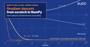
lr=0.1 converged after 57 iters | MSE=0.156107
lr=0.01 converged after 559 iters | MSE=0.156107Compared with 50,000 iterations that did not get there, the scaled data needs only 57 iterations at lr=0.1. The stability threshold of 0.9747 also matches: lr=1.0 exceeds the threshold and diverges (more slowly than lr=1.2 because it exceeds it only slightly), while 0.3 converges in just 15 iterations. The loss curve over iterations with lr=0.1:
MSE per iteration (lr=0.1): [16.7844, 10.7777, 1.9248, 0.3444, 0.1582, 0.1561] (iterations 0, 1, 5, 10, 20, 50)The learned parameters live in the scaled space, so they must be converted back to the original scale: w = w_z / sd and b = b_z - sum(w_z * mu / sd). Then compare with the closed-form solution:
GD parameters (converted to original scale): bias=1.0692, w=[ 0.1136 -0.2538]
lstsq parameters                           : bias=1.0692, w=[ 0.1136 -0.2538]
Max difference: 2.38e-06
The hand-written gradient descent matches the closed-form solution to about 1e-6. And scikit-learn's LinearRegression gives the same solution:
[sklearn LinearRegression] bias=1.0692, w=[ 0.1136 -0.2538]
MSE lstsq     : 0.156107
MSE sklearn   : 0.156107
Batch, mini-batch and stochastic gradient descent
The version above is batch gradient descent: every update uses all n samples. With millions of rows, each step is too expensive. Two common variants of gradient descent are summarized in Sebastian Ruder's survey An overview of gradient descent optimization algorithms (arXiv, 2016):
- Stochastic gradient descent (SGD): update after every single sample; steps are cheap and numerous, but the loss fluctuates.
- Mini-batch gradient descent: update after every small group (typically 32–256 samples); a balance between stability and speed that takes advantage of vectorized matrix multiplication, and the default choice when training neural networks.
def minibatch_gd(Zb, y, lr, epochs, batch, seed=0):
    r = np.random.default_rng(seed)
    theta = np.zeros(Zb.shape[1]); m = len(y)
    log = []
    for ep in range(epochs):
        idx = r.permutation(m)                 # shuffle every epoch
        for s in range(0, m, batch):
            bi = idx[s:s + batch]
            theta -= lr * grad(theta, Zb[bi], y[bi])
        log.append(mse(theta, Zb, y))
    return theta, log
--- SGD / mini-batch (z-score, 30 epochs) ---
batch (full) lr=0.1 MSE epoch 1=10.7777 | epoch 30=0.1561 | updates/epoch=1
mini-batch 32 lr=0.1 MSE epoch 1=0.8538 | epoch 30=0.1567 | updates/epoch=7
SGD (1 sample) lr=0.02 MSE epoch 1=0.1651 | epoch 30=0.1641 | updates/epoch=200A worthwhile observation: after 1 epoch, full batch has taken only one step (MSE 10.78), mini-batch is already down to 0.85, and SGD is already close to the bottom (0.165). But after 30 epochs, full batch reaches the bottom exactly (0.1561), mini-batch is slightly off (0.1567), and SGD still oscillates around the bottom (0.1641) because each step looks at a single noisy sample. To make SGD-style gradient descent converge close to the bottom, people decay the learning rate gradually; scikit-learn offers ready-made schedules such as invscaling and optimal for SGDRegressor. Note that lr=0.02 for SGD is a value I chose to be smaller to avoid excessive oscillation; it is a hyperparameter to tune, not a constant of the algorithm.
Gradient descent in the major libraries
- scikit-learn:
LinearRegressionuses the closed-form solution (SVD) and does not iterate;SGDRegressorandSGDClassifieruse SGD, suit very large datasets, and offerpartial_fitfor learning incrementally in batches (online/out-of-core). The documentation suggests starting withmax_iteraround 10^6 divided by the number of samples, and shuffling the data before training. - Deep learning: PyTorch and TensorFlow compute gradients automatically (automatic differentiation) instead of you deriving them by hand, and then use variants such as momentum or Adam on mini-batches. The core of gradient descent is still the
theta -= lr * gradloop you just wrote. - Logistic regression, linear SVM: the same framework; only the loss function and gradient change.
When not to implement gradient descent yourself
- Linear regression with a few tens of thousands of samples and a few dozen features:
LinearRegression(closed form) is fast, exact and needs no learning rate. - Strongly correlated features: the closed-form solution can be very sensitive to noise (the scikit-learn documentation warns that a nearly singular design matrix produces large variance); add regularization such as Ridge instead of just changing the optimizer.
- Real products: implementing gradient descent yourself is only for understanding and teaching. Use a well-tested library with numerically stable handling and edge cases covered.
- Non-convex loss (neural networks): gradient descent only guarantees reaching a local stationary point; that is the topic of the later deep learning articles in this series.
Common mistakes
- Not scaling features: a large condition number makes gradient descent slow and forces a very small learning rate, as in the example above.
- A wrong gradient while the loss still goes down: always run a gradient check with finite differences.
- Loss increases or becomes
inf/nan: the learning rate exceeds2/lambda_max; reduce it, usually by a factor of 3 to 10. - Scaling with statistics of the whole dataset (including the test set): this is data leakage; the Pipeline section in the next article fixes it at the root.
- Forgetting to convert parameters back to the original scale when reporting coefficients to business users: a coefficient of "0.52 on area" in z-score space does not mean 0.52 million per m².
- Forgetting to shuffle the data between epochs when using SGD or mini-batch, especially when the data is sorted by time or by label.
- Stopping after a fixed number of iterations without looking at the loss: add a tolerance-based stopping criterion such as the
tolabove.
Checklist
- Write the loss and gradient in vectorized form; verify the gradient with finite differences.
- Scale features with training-set statistics before running gradient descent.
- Choose a learning rate below
2/lambda_max; watch the loss curve over iterations. - Compare the result with the closed-form solution or
LinearRegressionto confirm the implementation is correct. - Use mini-batches when the data is large; decay the learning rate gradually if you need convergence close to the bottom.
- Convert parameters back to the original scale before interpreting them.
The full source code is in code/s7-10 (gd.py, stability.py, requirements.txt) and runs with python gd.py. This gradient descent code and every number in the article are real output from a run on an Apple M4, 16 GB; the data is synthetic, with random seed 42.
Next article
Machine learning with scikit-learn: Pipeline, cross-validation and tuning. Now that you understand the optimization mechanics underneath, we use scikit-learn to combine preprocessing and the model in a Pipeline, evaluate with cross-validation, and search for hyperparameters without leaking data.