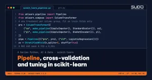
If you have ever standardized a whole table before splitting it into train and test sets, picked hyperparameters by watching the score on the test set, or forgotten to apply the right preprocessing when shipping a model, you have run into exactly the problems that scikit-learn was built to solve with three tools: Pipeline, cross-validation, and GridSearchCV. This article builds a customer churn prediction problem (simulated data) from start to finish: handling missing values, encoding categorical variables, scaling numeric variables, evaluating with stratified cross-validation, tuning hyperparameters, and then showing with real numbers how data leakage can turn pure noise into a "successful" model with an AUC of 0.87.
This article follows Linear regression and gradient descent: implementing it with NumPy, where we saw why features must be scaled, and What is machine learning: problems, data and the workflow of an AI project, which describes the overall workflow. Tabular data for scikit-learn is cleaned with the techniques in Cleaning crawled data with pandas: normalization, deduplication and data types. The environment used here: Python 3.10, scikit-learn 1.1.3, pandas 1.5, NumPy 1.23 (the stable versions at the time of writing). The APIs used in this article (Pipeline, ColumnTransformer, GridSearchCV, get_feature_names_out) are all available in scikit-learn 1.1.
Why you need a Pipeline in scikit-learn
According to the Pipelines and composite estimators documentation, Pipeline gives you three benefits: convenience and encapsulation (call fit and predict once for the whole chain of steps), joint parameter selection (grid search over the parameters of every step at the same time), and safety (it prevents statistics from the test data from leaking into the model during cross-validation, because the same training samples are used to learn both the transformers and the predictor). Every step except the last must be a transformer (having fit and transform); the last step can be a predictive model.
In other words, Pipeline turns a "workflow" into a single object that you can serialize, test, and deploy. That object is also the unit that cross-validation and tuning work on, so every learned operation (imputation, scaling, encoding, feature selection) automatically sees only the training part of each fold.
The data: customer churn (simulated)
We generate 1,500 customers with three numeric variables (months of usage, monthly fee, number of support calls), two categorical variables (plan, payment method), a binary label roi_bo (churned), and deliberately inject 90 missing values into each of cuoc_hang_thang (monthly fee) and goi_cuoc (plan). The logit formula sits right in the code so you can compare it with the coefficients learned at the end of the article. The data is entirely simulated and contains no personal information.
import numpy as np
import pandas as pd

rng = np.random.default_rng(7)
n = 1500
df = pd.DataFrame({
    "so_thang_su_dung": rng.integers(1, 60, n),
    "cuoc_hang_thang": rng.normal(250_000, 90_000, n).clip(50_000),
    "so_cuoc_goi_ho_tro": rng.poisson(1.5, n),
    "goi_cuoc": rng.choice(["co_ban", "tieu_chuan", "cao_cap"], n, p=[.5, .35, .15]),
    "thanh_toan": rng.choice(["chuyen_khoan", "the", "tien_mat"], n),
})
# the label comes from a logistic function: churn probability = 1 / (1 + exp(-logit))
logit = (-1.0 - 0.04 * df.so_thang_su_dung + 0.5 * df.so_cuoc_goi_ho_tro
         + 0.000004 * df.cuoc_hang_thang + (df.goi_cuoc == "co_ban") * 0.6
         + (df.thanh_toan == "tien_mat") * 0.4)
df["roi_bo"] = (rng.random(n) < 1 / (1 + np.exp(-logit))).astype(int)
# inject missing values: 90 random rows in each column
for c in ["cuoc_hang_thang", "goi_cuoc"]:
    df.loc[rng.choice(n, 90, replace=False), c] = np.nan
X, y = df.drop(columns="roi_bo"), df["roi_bo"]
scikit-learn 1.1.3
Shape: (1500, 5) | churn rate: 0.465
Missing values:
cuoc_hang_thang 90
goi_cuoc 90The first thing to do with scikit-learn, before any learning step, is to split off a test set and leave it alone. According to the Cross-validation guide, learning the parameters of a prediction function and then testing it on the same data is a methodological mistake. We use stratify=y to keep the label ratio the same in both parts:
X_tr, X_te, y_tr, y_te = train_test_split(X, y, test_size=0.2, stratify=y, random_state=42)train: (1200, 5) test: (300, 5)ColumnTransformer: one treatment per group of columns
Numeric variables need imputation (median) and then scaling; categorical variables need imputation (most frequent value) and then one-hot encoding. ColumnTransformer assigns each chain of transformations to its group of columns, then concatenates the results. The handle_unknown="ignore" parameter means that when the model meets a category it never saw during training, it does not raise an error but assigns all zeros.
so = ["so_thang_su_dung", "cuoc_hang_thang", "so_cuoc_goi_ho_tro"]
pl = ["goi_cuoc", "thanh_toan"]
pre = ColumnTransformer([
    ("so", make_pipeline(SimpleImputer(strategy="median"), StandardScaler()), so),
    ("pl", make_pipeline(SimpleImputer(strategy="most_frequent"),
                         OneHotEncoder(handle_unknown="ignore")), pl),
])
pipe = Pipeline([("pre", pre), ("clf", LogisticRegression(max_iter=1000))])
The scikit-learn naming convention step__parameter (two underscores) gives access to nested parameters at any level; this is also how you declare a search grid:
Parameter names in step__parameter form: ['pre__so__simpleimputer__strategy', 'pre__pl__onehotencoder__handle_unknown', 'clf__C']The string pre__so__simpleimputer__strategy goes through the pre step (the ColumnTransformer), the so branch, the imputer simpleimputer (a name that make_pipeline generates automatically from the lowercase class name), and finally the strategy parameter.
Stratified cross-validation in scikit-learn: a more reliable estimate
A single train/validation split in scikit-learn gives a score that depends on the luck of the split. K-fold cross-validation divides the training set into k parts, trains on k−1 parts, evaluates on the remaining part, and then averages the results. For classification problems, use StratifiedKFold so that each fold keeps class proportions close to the whole set; the scikit-learn documentation illustrates class-ratio preservation with an example of 45 negative samples and 5 positive samples. With a rare class like that, an unstratified random split can produce a fold with very few positive samples or none at all, while StratifiedKFold guarantees that every fold contains both classes. If you pass cv=5 to a classifier, scikit-learn already uses StratifiedKFold (without shuffling); we declare it explicitly so we can set shuffle=True and random_state.
cv = StratifiedKFold(n_splits=5, shuffle=True, random_state=0)
sc = cross_val_score(pipe, X_tr, y_tr, cv=cv, scoring="roc_auc")
res = cross_validate(pipe, X_tr, y_tr, cv=cv,
                     scoring=["roc_auc", "average_precision", "f1"],
                     return_train_score=True)
[CV 5-fold] ROC AUC per fold: [0.708 0.707 0.754 0.731 0.768] | mean 0.733 ± 0.024
train_roc_auc 0.740
test_roc_auc 0.733
test_average_precision 0.714
test_f1 0.642There are two things to read from this scikit-learn result. First, the scores across folds range from 0.707 to 0.768; a single split could give you a number anywhere in that range, so reporting "mean ± standard deviation" is the honest approach. Second, the training AUC (0.740) is close to the test AUC (0.733): a simple linear model on this data does not overfit, and the problem is that the data is very noisy, not that the model is too complex. The scikit-learn cross_validate function differs from cross_val_score in that it allows several metrics at once and returns fit/score times; training scores are off by default, and we turn them on with return_train_score=True to diagnose overfitting.
Data leakage: an experiment with pure noise
Data leakage when using scikit-learn happens when information that is not available at prediction time gets into training. The Common pitfalls and recommended practices page stresses splitting train and test before any preprocessing step and never passing test data into fit or fit_transform. To see how harmful this is, we create data that we know for certain contains no signal: 100 samples, 2,000 random features, random labels. The correct AUC should be around 0.5.
from sklearn.feature_selection import SelectKBest, f_classif
from sklearn.linear_model import LogisticRegression
from sklearn.model_selection import cross_val_score
from sklearn.pipeline import make_pipeline

rng2 = np.random.default_rng(0)
Xn = rng2.normal(size=(100, 2000)); yn = rng2.integers(0, 2, 100)
# WRONG: select the 20 "best" features on the whole dataset, then cross-validate
Xs = SelectKBest(f_classif, k=20).fit_transform(Xn, yn)
leak = cross_val_score(LogisticRegression(max_iter=1000), Xs, yn, cv=5, scoring="roc_auc")
# RIGHT: put the feature selection step inside the Pipeline
ok_pipe = make_pipeline(SelectKBest(f_classif, k=20), LogisticRegression(max_iter=1000))
good = cross_val_score(ok_pipe, Xn, yn, cv=5, scoring="roc_auc")
[Leakage] pure noise data, 100 samples x 2000 features
feature selection BEFORE CV (wrong): mean AUC = 0.867
feature selection INSIDE Pipeline : mean AUC = 0.578The wrong approach reports an AUC of 0.867 on data that contains no information at all. The feature selection step has "seen" the labels of every sample, including samples that later end up in the test fold, so it picks exactly the columns that happen to correlate with the labels. Inside a Pipeline, that step learns only on the training part of each fold, and the result falls to 0.578, close to chance (with 100 samples this number still fluctuates, so do not expect exactly 0.5).
This is also the spirit of the example in the scikit-learn documentation with 200 samples and 10,000 random features; the problem is analyzed in the classic book The Elements of Statistical Learning (Hastie, Tibshirani, Friedman), section 7.10.2, on selecting features before cross-validation. The lesson: every step that has a fit must be inside the Pipeline, including feature selection, dimensionality reduction, and class balancing.
Hyperparameter tuning with scikit-learn GridSearchCV
Hyperparameters are parameters that are not learned from data but set beforehand, such as C in logistic regression (the strength of regularization; the smaller C is, the stronger the regularization). According to the Tuning the hyper-parameters documentation, GridSearchCV tries every combination in the grid, while RandomizedSearchCV samples a fixed number of combinations from the parameter space. Because scikit-learn search runs on a Pipeline, we can also tune the preprocessing steps, here the imputation strategy, mean or median.
grid = {"clf__C": [0.01, 0.1, 1, 10, 100],
        "pre__so__simpleimputer__strategy": ["mean", "median"]}
gs = GridSearchCV(pipe, grid, cv=cv, scoring="roc_auc", n_jobs=-1)
gs.fit(X_tr, y_tr)
print(gs.best_params_, gs.best_score_)
print(gs.score(X_te, y_te))
[GridSearchCV] best_params_: {'clf__C': 0.1, 'pre__so__simpleimputer__strategy': 'median'}
[GridSearchCV] best CV AUC: 0.734
param_clf__C param_pre__so__simpleimputer__strategy mean_test_score rank_test_score
0.1 median 0.733942 1
0.1 mean 0.733859 2
0.01 mean 0.733677 3
0.01 median 0.733551 4
[Test set, touched once] AUC = 0.790Three points are worth noting. Point one: the top four configurations differ by less than 0.0004 AUC, far smaller than the standard deviation across folds (0.024). This means that on this data, mean versus median, or C=0.01 versus 0.1, are configurations that cross-validation cannot tell apart; do not interpret "median wins" as a finding. (This is a practical way to read the results, not a statistical test, because the configurations share the same folds.)
Point two: GridSearchCV defaults to refit=True, meaning that after choosing the best combination it retrains on the whole training set, and gs.score uses that model.
Point three: the score on the test set (0.790) is higher than the cross-validation score (0.734). The test set has only 300 samples, so it fluctuates too; the gap comes from the luck of a single split and does not prove the model is better than expected. We touch the test set exactly once, after every choice has been finalized; if you repeat "look at test, tweak, look at test", the test set becomes a validation set and the number loses its value. The documentation recommends splitting into a development set (fed into GridSearchCV) and an evaluation set for computing the final metric.
Swapping the model in the grid and using RandomizedSearchCV
Because the clf step is also a parameter of the Pipeline, we can put several kinds of models into the same search using a list of dictionaries, where each dictionary corresponds to one model and its own parameters. For a continuous parameter like C, declare a distribution (here SciPy's loguniform) instead of listing a few values; RandomizedSearchCV samples from that distribution, and increasing n_iter is enough to try more values without rebuilding the grid. This is also the approach the documentation recommends for continuous parameters.
space = [
    {"clf": [LogisticRegression(max_iter=1000)], "clf__C": loguniform(1e-3, 1e2)},
    {"clf": [RandomForestClassifier(random_state=0, n_jobs=-1)],
     "clf__n_estimators": [100, 200, 300], "clf__max_depth": [3, 5, 8, None]},
]
rs = RandomizedSearchCV(pipe2, space, n_iter=12, cv=cv, scoring="roc_auc", random_state=0)
rs.fit(X_tr, y_tr)
[RandomizedSearchCV] winning model: LogisticRegression | CV AUC 0.734
parameters: {'clf': 'LogisticRegression', 'clf__C': 0.030737817853626094}
test set AUC: 0.789
best CV score per model:
LogisticRegression 0.734 (6 configurations tried)
RandomForestClassifier 0.718 (6 configurations tried)The scikit-learn random forest does not win: its best CV score is 0.718, lower than the 0.734 of logistic regression (each model was tried on 6 of the 12 sampled configurations). This makes sense because we generated the labels from a logistic function, so the linear model matches the true structure exactly; on real data you will not know that in advance, which is exactly why you should compare with cross-validation instead of guessing. A rule of thumb follows: start with a simple model as a baseline, and move to a complex model only when CV shows it helps.
Reading the final model of a scikit-learn Pipeline
Because the preprocessing lives inside the scikit-learn Pipeline, we get the feature names after transformation with get_feature_names_out() and then read the coefficients by pairing them with the coef_ of the clf step:
[Logistic regression coefficients, standardized/one-hot features]
  so__so_thang_su_dung                     -0.606
  so__so_cuoc_goi_ho_tro                   +0.585
  pl__goi_cuoc_co_ban                      +0.351
  pl__goi_cuoc_tieu_chuan                  -0.283
  so__cuoc_hang_thang                      +0.261
  pl__thanh_toan_tien_mat                  +0.133
The direction and magnitude match how we generated the data: customers who stay longer churn less, and customers who call support often or are on the basic plan churn more. The learned coefficients are on standardized features, so they cannot be compared directly with the coefficients in the data-generating formula (which are on the original scale).
To compare them, multiply the true coefficient by the column's standard deviation: -0.04 × 16.9 ≈ -0.68 for months of usage, 0.5 × 1.19 ≈ +0.59 for support calls, 0.000004 × 90,562 ≈ +0.36 for the monthly fee.
The learned values (-0.606, +0.585, +0.261) have the same direction and the same order of magnitude; the gap, clearest for the monthly fee, comes from regularization (C=0.1) shrinking the coefficients toward 0 and from the sampling noise of 1,200 rows. Because the numeric variables are standardized, comparing magnitudes between numeric variables is valid. One-hot coefficients are compared against the remaining categories of the same column. Do not interpret coefficients as causal relationships: the model only says which variables go together with the label.
scikit-learn in practice: reusable patterns
- One object to deploy: with scikit-learn, save the whole
Pipeline(for example withjoblib.dump) instead of saving the scaler and the model separately, so that at prediction time you cannot apply the wrong order or the wrong parameters. Load model files only from trusted sources, because pickle can execute arbitrary code when loading. - Columns by data type: with wide tables, use
make_column_selector(dtype_include="number")instead of listing columns by hand; theColumnTransformerdocumentation describes how to select columns by dtype or name pattern. - Skip a step during search: set a preprocessing step to
"passthrough"in the grid to check whether that step really helps (for example with or without scaling). - Stratified and grouped splits: for time-ordered data use
TimeSeriesSplit, and for data with many rows from the same customer useGroupKFold; both are covered in the cross-validation documentation. Random shuffling in these cases causes leakage. - Multiple metrics: in scikit-learn, pass
scoringas a list together withrefit="roc_auc"when you need to track several metrics; the next article on model evaluation goes deeper into choosing the right metric for imbalanced data.
When not to use a scikit-learn Pipeline or broad tuning
- Too much tuning on small data: the larger the search grid, the more likely the top score is just luck. With 1,200 samples and a 0.0004 difference as above, tuning only costs time; if you need an honest performance estimate after tuning, use nested cross-validation (see the Nested versus non-nested cross-validation example).
- Heavy preprocessing outside scikit-learn: text transformations, images, or features from external APIs are usually separated from the Pipeline (built in advance and saved), as long as they do not use statistics from the test set.
- Large data that does not fit in memory: beyond plain scikit-learn, consider estimators with
partial_fit(such asSGDClassifier) or other tools, becausePipelinewith cross-validation duplicates data across folds. - Exploration only: with scikit-learn, if you just want a quick look at the data, a full Pipeline is overkill; but as soon as a number goes into a report, switch to a Pipeline.
Common mistakes
- Fitting the scaler or imputer on the whole dataset before splitting: put it in a Pipeline.
- Selecting features before cross-validation: the experiment above shows an AUC of 0.867 on pure noise.
- Using the test set to choose hyperparameters: use
cv_results_and touch the test set only once. - Drawing conclusions from differences smaller than the standard deviation across folds: report both the mean and the standard deviation.
- Forgetting
stratifywhen labels are imbalanced, or forgettingshufflewhen data is sorted by label; the default is no shuffling. - Wrong parameter names in the grid:
clf__C, notC; usepipe.get_params().keys()to look them up. - Not pinning library versions: default parameters and warning values change between releases; write a
requirements.txt(included incode/s7-11) so you can reproduce the results. - Forgetting
handle_unknown="ignore"inOneHotEncoder, which causes errors when a new category appears in production.
Checklist
- Split off a stratified test set before any learning step.
- Put every step that has a
fitinto one scikit-learnPipelinewith aColumnTransformer. - Evaluate with scikit-learn stratified cross-validation, and report mean ± standard deviation and the training score.
- Tune with scikit-learn
GridSearchCVorRandomizedSearchCVon the Pipeline; compare the differences with the standard deviation. - Start with a simple baseline; increase complexity only when CV shows it helps.
- Touch the test set once; save the whole Pipeline and pin library versions.
The full source code is in code/s7-11 (pipeline_demo.py, output.txt, requirements.txt); run it with python pipeline_demo.py in a venv. All numbers are real output from running with Python 3.10, scikit-learn 1.1.3, pandas 1.5.1, and NumPy 1.23.4 (pinned in requirements.txt); the data is simulated with fixed seeds, so rerunning gives the same results (small differences in the last digits may appear if you change the BLAS or library version). The process uses about 150 MB of RAM.
Next article
Model evaluation for classifiers: precision, recall, ROC and imbalanced data. We have just used ROC AUC, average precision, and F1 almost only for comparison; the next article goes into what each metric means, why accuracy is misleading on imbalanced data, and how to choose a decision threshold based on business cost.