Two models with the same algorithm can differ by anywhere from a few points to dozens of AUC points purely because of how the input data is represented, as the experiments below show. That is why feature engineering, the work of turning raw table columns into features a model can learn from, is worth investing in for machine learning projects on tabular data. This article does feature engineering on an order-return prediction problem (simulated data, 6,000 orders) and walks through four concrete tasks: scaling numeric variables, encoding a categorical variable with 80 values, creating time features, and most importantly, spotting data leakage before it turns a useless model into an "excellent" one.
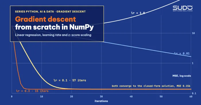
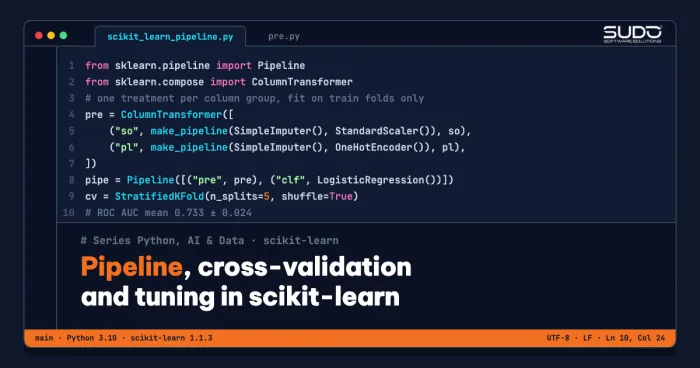
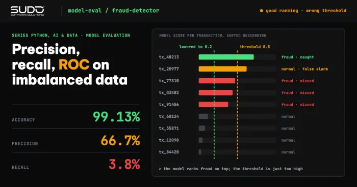
This article follows Model evaluation for classifiers: precision, recall, ROC and imbalanced data and Machine learning with scikit-learn: Pipeline, cross-validation and tuning; we reuse Pipeline and ColumnTransformer from there. The reason scaling often helps gradient descent converge faster is covered in Linear regression and gradient descent: implementing it with NumPy. Environment: Apple M4, 16 GB, Python 3.10, scikit-learn 1.2.0, pandas 1.5.3, NumPy 1.24.1; every API used here has been available since scikit-learn 1.1.
What feature engineering is and why it decides model quality
According to the book Feature Engineering and Selection by Max Kuhn and Kjell Johnson (2018), re-representing the predictors is a real modeling step, not a side chore of cleanup. The authors themselves warn that the process can also cause overfitting, because the number of possible representations is huge. The practical consequence: every time we "try one more feature" we look at the data and make a choice, so we must measure with cross-validation, not intuition.
For tabular data, feature engineering revolves around four groups: numeric variables (scaling, log), categorical variables (one-hot, ordinal, target encoding), time (splitting out hour, weekday, week) and missing values, where the missingness itself is sometimes the signal. The rule that runs through all feature engineering: any transformation that learns statistics from the data must learn them on the training set only; violating that is data leakage.
Sample data for feature engineering: e-commerce orders
We generate 6,000 orders with order value (VND, right-skewed), item count, delivery district (80 values, Zipf-like frequency: a few very busy districts and many rare ones), sales channel, size, order hour, order timestamp, and days since the previous purchase (missing for new customers). The label is whether the order was returned, generated from a noisy logistic function, so we know for certain which variables carry real signal. The data is entirely simulated and contains no personal information.
[1] Data: (6000, 8) | return rate: 0.400
Districts: 80 | rarest district: 19 orders | busiest: 783
Missing so_ngay_tu_lan_mua: 36.2%
Skew of gia_tri: 4.48 -> after log1p: 0.00
We use a stratified 75/25 split; every "CV AUC" number below is the mean ± standard deviation of 5-fold cross-validation on the 4,500 training orders only.
Feature engineering for numeric variables: when scaling helps
The Preprocessing data page in the scikit-learn documentation describes StandardScaler (subtract the mean, divide by the standard deviation), MinMaxScaler (rescale to the range [0, 1]) and RobustScaler (uses the median and interquartile range, robust to outliers). In feature engineering, scaling does not always improve the score. We test it on two variables, gia_tri (on the order of hundreds of thousands) and so_san_pham (a few units), with two models of different nature:
pipe = make_pipeline(ColumnTransformer([("n", tf, ["gia_tri", "so_san_pham"])]), LogisticRegression(max_iter=3000))
# tf in turn: "passthrough", StandardScaler(), RobustScaler(), log1p + StandardScaler
no scaling 0.6691 ± 0.0155
StandardScaler 0.6762 ± 0.0133
RobustScaler 0.6762 ± 0.0133
log1p + StandardScaler 0.6831 ± 0.0163
Same 2 variables with k-NN (k=25), where distance depends directly on scale:
no scaling 0.6416 ± 0.0179
StandardScaler 0.6514 ± 0.0208
log1p + StandardScaler 0.6532 ± 0.0223
lbfgs iterations (no scaling): 5
lbfgs iterations (StandardScaler): 6
L2 penalty makes the solution scale-dependent; with C=0.001 (strong penalty), Logistic Regression CV AUC:
C=0.001, no scaling 0.6691 ± 0.0155
C=0.001, StandardScaler 0.6728 ± 0.0130
Example: mean gia_tri in train = 332719, standard deviation = 378333 (mean_/scale_ of the scaler)Three things can be read from the real numbers in this feature engineering step. First, for logistic regression, StandardScaler and RobustScaler give identical AUC to four digits (0.6762), while the unscaled version is slightly lower (0.6691). LogisticRegression applies an L2 penalty with C=1 by default, so the optimal solution depends on feature scale; the two scalers matching comes from the fact that they bring the features to an equivalent scale and the L2 penalty is weak relative to 4,500 samples. The C=0.001 rows show the opposite direction: with a strong penalty, the two scaling choices diverge (0.6691 versus 0.6728).
The lbfgs iteration counts (5 versus 6) in this scikit-learn 1.2.0 run do not show a speed advantage from scaling, so we draw no conclusion about convergence speed from this run; this is a place where iteration counts depend on the version and the solver's stopping criterion.
Second, k-NN is sensitive to scale because distance is dominated by the variable with the largest magnitude: AUC rises from 0.6416 to 0.6514. Third, a log1p transform on the right-skewed variable (skew 4.48 down to 0.00) adds a little more, but the difference of about 0.007 is smaller than the standard deviation across folds, so it should not be over-interpreted.
The rule for numeric feature engineering: use scaling with distance-based models (k-NN, SVM, K-Means) and with regularized linear models (L2 penalty makes the solution scale-dependent) or gradient-optimized ones; it is not needed for decision trees and boosted tree models (covered in the next article of the series). A log transform helps when the relationship with the label is roughly multiplicative and the distribution is heavily skewed, like order value.
Feature engineering for high-cardinality categorical variables
The quan variable has 80 values, from a district with only 19 orders to one with 783. We compare the encoding approaches in feature engineering, each placed in the same ColumnTransformer with the remaining variables (log of value, item count, size in the order S < M < L < XL, one-hot sales channel, a "new customer" flag):
OneHotEncoder(handle_unknown="infrequent_if_exist", min_frequency=60) # variant that groups rare districts without district 0.7236 ± 0.0242
OrdinalEncoder (codes 0..79) 0.7247 ± 0.0234
OneHotEncoder (80 columns) 0.7549 ± 0.0174
OneHot + min_frequency=60 0.7389 ± 0.0167 (18 columns, 63 rare districts grouped)In feature engineering, OrdinalEncoder assigns codes 0 to 79 in alphabetical order, an order that is meaningless for delivery districts; a linear model treats it as a straight line and learns almost nothing (0.7247 versus 0.7236 when the variable is dropped entirely). Use ordinal encoding only for variables with a real order such as size, or for tree models. OneHotEncoder gives each district a binary column and lifts AUC to 0.7549. With handle_unknown="ignore", an unseen district at prediction time becomes an all-zero vector instead of crashing the pipeline.
When cardinality reaches the thousands, feature engineering for categorical variables has to account for matrix size: one-hot produces a wide matrix. Since scikit-learn 1.1, min_frequency groups rare values into one "infrequent" column. Here min_frequency=60 groups 63 rare districts, leaving 18 columns, in exchange for losing information about each rare district: AUC drops to 0.7389. This is a tunable trade-off, and it also buys stability: for a district with only 19 orders, the learned coefficient is very noisy.
Target encoding: powerful but easy to break
Target encoding is a feature engineering technique that replaces each value with the mean label of its group. The original paper by Micci-Barreca (SIGKDD Explorations, 2001) proposes blending the group mean with the global mean according to group size, so small groups are not estimated erratically. The smoothing formula we implement is (n·group_mean + m·global_mean) / (n + m), where m is the strength of the pull toward the overall mean. We write a small class with an out-of-fold option: each training row is encoded using only statistics from the other folds.
for a, b in KFold(5, shuffle=True, random_state=0).split(c):
    mp, mu = fit_map(c.iloc[a], t[a])                    # statistics only from the other folds
    out[b] = c.iloc[b].map(mp).fillna(mu).to_numpy()     # fold b is encoded with them
To see the consequence, we create a nearly unique "customer code" (about 3,000 values for 4,500 rows, carrying no information about the label) and let HistGradientBoostingClassifier learn from that encoded feature alone:
[3b] Target encoding for the nearly unique variable 'ma_khach' (customer ID: ~3,000 values for 4,500 rows, no information)
  naive (m=1, in-sample)           AUC train = 0.914 | AUC test = 0.503
  out-of-fold (cross-fitting)      AUC train = 0.579 | AUC test = 0.472
Naive encoding gives a training AUC of 0.914 on a pure-noise feature, then collapses to 0.503 (random) on the test set: the model merely memorizes each row's label through the feature. The out-of-fold version gives a training AUC of 0.579, close to random, which matches the truth that this variable is useless. The key point: a feature computed from the label must be computed without using that row's own label.
For a variable with real signal and large group sizes, the result is very different:
[3c] Target encoding of district (80 values, real signal) with LogisticRegression on the full table
  in-sample, m=20      AUC train = 0.7706 | AUC test = 0.7607
  out-of-fold, m=20    AUC train = 0.7528 | AUC test = 0.7591
  (for comparison) OneHot 80 columns:  AUC train = 0.7737 | AUC test = 0.7629
Each district has about 56 orders on average, so leakage is small: the test AUCs are close and one-hot is not worse (0.7629). Only the training AUC column differs: the in-sample version is more optimistic, and the out-of-fold version is closer to the test score. The honest conclusion: target encoding is worth using when cardinality is very large (postal codes, product codes); with a few dozen values, one-hot is good enough.
Feature engineering for time: cyclical variables and component extraction
Order hour is a cyclical variable: 11 p.m. and midnight are one hour apart, but on the 0..23 number line they are 23 units apart. A common feature engineering approach is to represent it as a sin and cos pair of 2π·hour/24, so the hour sits on a circle. We compare three approaches on the same table:
np.c_[np.sin(2 * np.pi * h / 24), np.cos(2 * np.pi * h / 24)] # h = order hour, 0..23 raw gio_dat (0..23), linear 0.7281 ± 0.0206
sin/cos of gio_dat 0.7507 ± 0.0209
OneHot 24 hours 0.7488 ± 0.0198The raw hour barely helps (0.7281 versus 0.7236 without it), while sin/cos raises it to 0.7507 with just two columns, on par with 24-column one-hot (0.7488). This transformation suits our data because the label was generated from the cosine of the hour; on real data, plot the label rate by hour before choosing. The same applies to weekday and month; for a full ngay_dat timestamp, split out the weekday, week, weekend flag and holidays instead of feeding in the raw timestamp.
Data leakage in feature engineering: four common forms
The Common pitfalls and recommended practices section of scikit-learn defines data leakage as using information that is not available at prediction time to build the model, leading to overly optimistic performance estimates, and states the rule: never call fit on test data. We reproduce four forms of leakage in feature engineering with real numbers, because mishandled feature engineering is the most common source of leakage.
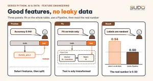
Form 1: selecting features on the whole dataset
That documentation uses an example with 200 samples, 10,000 random features and random labels. We redo it in the same spirit: no model should exceed 0.5 accuracy.
SelectKBest(f_classif, k=25).fit(Xn, yn)     # WRONG: selects features using the test set's labels too
make_pipeline(SelectKBest(f_classif, k=25), LogisticRegression(max_iter=1000)).fit(Xa, ya)   # RIGHT
Random labels, 10,000 noise features, 200 samples (accuracy should be ≈ 0.5)
- select features on the WHOLE data, then split: test accuracy = 0.94
- Pipeline (selection on each training split): test accuracy = 0.50
- 5-fold CV, select first: 0.88 | 5-fold CV with Pipeline: 0.53An accuracy of 0.94 on pure noise is a number convincing enough for an entire board of directors, and it is completely wrong. When the feature selection step sits inside a Pipeline, it learns only on the training part of each fold and the result returns to the random level, 0.50 and 0.53, matching the truth.
Form 2: scaling or imputing before the split
This form is milder but the most common in feature engineering. The mean order value is 332,719 on the training set and 333,553 on the whole data. To measure the harm, we compare k-NN on the two numeric variables when StandardScaler is fit on the whole data (including the test set) versus on the training set only:
  k-NN, scaler fit on ALL data (train + test)   AUC test = 0.6792
  k-NN, scaler fit on train only                AUC test = 0.6801
The two numbers are nearly equal (the leaky version is even slightly lower due to noise): with 6,000 rows and a simple scaling step, this leakage is not measurable. That does not mean it is safe. It becomes dangerous when the preprocessing step is stronger (feature selection as in form 1, PCA, target encoding), so always use a Pipeline.
Form 3: features known only after the event
We add a da_hoan_tien column (whether the order already has a refund slip), a column created after the order was returned:
  Features ['gia_tri', 'so_san_pham']                    AUC test = 0.6671
  Features ['gia_tri', 'so_san_pham', 'da_hoan_tien']    AUC test = 0.9494
  (da_hoan_tien is known only after the order has been returned -> it will not exist in real prediction)
AUC jumps from 0.6671 to 0.9494, but when predicting a new order, this column does not exist yet. This kind of leakage lives in the business process, not in the code. The test question for every column: "at the moment we need to predict, do we already have this value?" A warning sign is a single feature with unbelievably high importance.
Form 4: looking into the future when aggregating over time
An aggregate feature such as "district return rate in the week" feels very natural for transaction data. But if computed with groupby(...).transform("mean"), each order is computed together with the orders that come after it in the week, and with its own label. The correct version uses only orders that happened earlier, smoothed toward the overall rate:
g = d2.groupby(["quan", "tuan"])["y"]
d2["ty_le_tuan_ca_tuan"] = g.transform("mean")                       # WRONG: includes the current order and later ones
cum_sum = g.cumsum() - d2["y"]; cum_cnt = g.cumcount()               # RIGHT: only orders that happened earlier in the week
d2["ty_le_tuan_qua_khu"] = ((cum_sum + 0.4 * 5) / (cum_cnt + 5))
[6] Temporal leakage: district return rate in the week
only gia_tri, so_san_pham AUC test (last 25%) = 0.6550
+ ty_le_tuan_qua_khu AUC test (last 25%) = 0.6599
+ ty_le_tuan_ca_tuan AUC test (last 25%) = 0.8365
Average orders per (district, week): 3.6Because each (district, week) group has only about 3.6 orders, the "whole-week mean" nearly contains the row's own label, so AUC shoots up to 0.8365, while the past-only version barely changes (0.6599 versus 0.6550, as expected because the real signal here is weak). The lesson: time-aggregated features must be computed "up to time t", and when the data has a time dimension, split train/test by time.
Putting feature engineering into a leak-free Pipeline
Three principles turn the feature engineering above into a habit for every future feature engineering project: split the data before any learning step; put every transformation that has a fit into a Pipeline and ColumnTransformer so cross-validation relearns from scratch in each fold; treat every feature derived from the label or from the future as a suspect.
When not to do more feature engineering
- Too little data: feature engineering that adds columns only adds room to overfit, especially when the number of columns approaches the number of rows.
- Tree models: scaling-style feature engineering is redundant, because trees do not need scaling and are insensitive to monotonic transformations such as log; put the effort into business features (ratios, time gaps, per-customer aggregates).
- Mass automatic feature engineering: it easily creates spurious correlations and is hard to explain; every feature should have a business hypothesis.
Common mistakes and a feature engineering checklist
Common mistakes: calling fit_transform on the test set; forgetting handle_unknown so the pipeline crashes on a new value; using ordinal encoding for an unordered variable with a linear model or k-NN; target encoding without out-of-fold, especially for nearly unique variables like customer codes; splitting randomly on time-based data and then being surprised that the model is poor after deployment.
Checklist:
- Feature engineering that learns (scalers, encoders, feature selection) runs only after the train/test split, split by time if the data has a time dimension.
- Every step sits inside a
Pipeline; evaluate with stratified cross-validation and touch the test set once. - Numeric variables: scale for distance-based or gradient-based models; log for right-skewed variables.
- Categorical variables: one-hot with
handle_unknownandmin_frequency; ordinal only for ordered variables; target encoding always out-of-fold. - Cyclical variables (hour, weekday, month): sin/cos or one-hot, not raw numbers.
- For each new feature, ask: is it available at prediction time, and does it use the label or future data?
The full source code is in code/s7-13 (fe_demo.py, output.txt, requirements.txt); run it with python fe_demo.py in a venv. All figures are real output on an Apple M4, 16 GB, Python 3.10, scikit-learn 1.2.0, pandas 1.5.3; the data is simulated with a fixed seed, so rerunning gives the same results on the same versions (other library versions may differ in the last decimal digits).
Next article
Gradient boosting with XGBoost and LightGBM: when it beats deep learning. Once feature engineering is done and you have a clean feature table, the next article introduces boosted tree models, which often give the best results on tabular data, and compares them honestly with neural networks.