A credit-scoring model rejects a customer's loan application. The customer asks why, the risk team asks whether the model relies on sensible data, and the regulator asks for evidence. With gradient boosting, "because hundreds of decision trees said so" is not an answer. SHAP (SHapley Additive exPlanations) answers by splitting the gap between one customer's prediction and the average prediction across the features, using a definition grounded in game theory. This article uses exactly that problem (simulated data, 10,000 customers) to implement Shapley values by hand, check the additivity property numerically, compare SHAP with two other importance measures, and point out where SHAP is easy to misread.
It follows Gradient boosting with XGBoost and LightGBM: when it beats deep learning, which concluded that gain-based importance is not reliable enough. How correlated features and data leakage affect interpretation is covered in Feature engineering for tabular data: encoding, scaling and data leakage. Environment: Apple M4, 16 GB, Python 3.12. Every API used here (TreeExplainer, KernelExplainer, shap.Explanation, shap.plots.waterfall, beeswarm, scatter) has existed since shap 0.41 (June 2022) and XGBoost 1.7 (October 2022), both released before March 2023.
What SHAP is and where it comes from
Shapley values come from cooperative game theory. According to the Shapley values chapter of Christoph Molnar's Interpretable Machine Learning book, each feature value of an instance is a "player", the payout is the prediction minus the average prediction, and a feature's contribution is the change in prediction when it is added to a set of features, averaged with weights over all possible feature sets. The method satisfies four axioms: efficiency (the contributions add up to the prediction minus the average), symmetry, dummy (a feature that never changes the prediction gets zero) and additivity.
The paper A Unified Approach to Interpreting Model Predictions by Scott Lundberg and Su-In Lee (NIPS 2017) named this framework SHAP. They showed that a class of "additive feature attribution methods" has a unique solution with a set of desirable properties, and they unified six existing explanation methods under the same framework. The practical result: a SHAP explanation of a single prediction always has the form
f(x) = base_value + SHAP(feature 1) + SHAP(feature 2) + ... + SHAP(feature p)where the base value is the average prediction. A positive SHAP value pushes the prediction above the average, and a negative one pulls it below. The unit matters: for a classifier such as XGBoost, SHAP values are on the log-odds scale by default, not the probability scale. We will see the consequences later.
Data and model
We generate 10,000 borrowers with six columns: age, monthly income, total spending, months of employment, debt-to-income ratio and number of late payments. The label is default, generated from a logistic function in which tong_chi_tieu (total spending) has no direct effect but is built as roughly 55 to 75% of income plus noise. We do this on purpose so we can later check how SHAP handles correlated features. The data is entirely simulated and contains no personal information.
[1] Data: (10000, 6) | default rate: 0.215 | corr(thu_nhap, tong_chi_tieu) = 0.96
    XGBoost AUC test = 0.7265
The model is an XGBClassifier with 300 trees, depth 3 and learning rate 0.05, trained on 75% of the data; the AUC on the remaining 25% is 0.7265.
TreeExplainer: explaining one prediction and checking additivity
For tree models, SHAP has a dedicated algorithm. The paper Consistent Individualized Feature Attribution for Tree Ensembles (Lundberg, Erion, Lee) presents an exact tree algorithm that is exponentially faster than brute force, introduces SHAP interaction values, and notes that the implementation is integrated into XGBoost and LightGBM. Using it takes only a few lines:
expl = shap.TreeExplainer(model)
sv = expl.shap_values(X_te)                      # matrix (rows, features), log-odds scale
margin = model.predict(X_te, output_margin=True)
np.abs(expl.expected_value + sv.sum(1) - margin).max()
[2] TreeExplainer and the additivity property (local accuracy), output in log-odds
base value E[f(x)] (log-odds) = -1.2989 -> probability 0.214
max error |base + sum of SHAP - model log-odds| over 2500 rows = 3.34e-06The base value is -1.2989 log-odds, which corresponds to a probability of 0.214, close to the dataset's default rate of 0.215. Across all 2,500 test customers, the base plus the sum of SHAP values matches the model's log-odds with a maximum error of 3.34e-06, which is single-precision floating-point error in XGBoost. This is the local accuracy property, and we verify it numerically instead of trusting the documentation. Now take a customer from the highest-risk group:
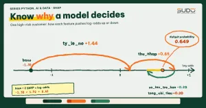
    Customer #7535 (in the high-risk group): predicted default probability = 0.649
      ty_le_no           = 0.776        SHAP = +1.441
      thu_nhap           = 1.314e+07    SHAP = +0.654
      so_lan_tre_han     = 0            SHAP = -0.394
      tong_chi_tieu      = 5.66e+06     SHAP = +0.199
      tuoi               = 35           SHAP = +0.009
      so_thang_lam_viec  = 67           SHAP = +0.007
      base -1.299 + sum of SHAP +1.915 = +0.617 (model log-odds: +0.617)
Read it like a report for the risk team: this customer has a 64.9% default probability versus a 21.4% average. The strongest factor pushing risk up is the debt ratio of 0.776 (+1.441), followed by an income of 13.1 million VND, lower than typical (+0.654). Never having been late pulls risk down (-0.394), while age and months of employment contribute almost nothing.
One point stands out: tong_chi_tieu receives +0.199 even though the data generator gave it no direct effect. We return to this in the section on correlated features.
Computing Shapley values from the definition to see that SHAP is not magic
We check by implementing the definition itself. With p = 6 features there are only 26 = 64 subsets, so brute force is feasible. The value function v(S) is the average prediction when the features in S take the current customer's values and the remaining features are drawn from 100 background rows:
def value(S, x):
    B = bg.copy()                                   # bg: 100 background rows from the training set
    for c in S: B[c] = x[c]
    return model.predict(B, output_margin=True).mean()

# for each feature c: phi[c] = sum over all subsets S of the remaining features of
#   weight * (v(S ∪ {c}) - v(S)),  weight = |S|! (p-|S|-1)! / p!
[3] Shapley value from the definition (brute force over all subsets) vs shap, interventional, 100-row background
6 features -> 64 subsets; brute force: 0.09s | TreeExplainer: 0.0023s
tuoi brute force = +0.01681 | shap = +0.01681 | diff = 2.3e-08
thu_nhap brute force = +0.71914 | shap = +0.71914 | diff = 7.3e-08
tong_chi_tieu brute force = +0.16540 | shap = +0.16540 | diff = 1.3e-07
so_thang_lam_viec brute force = +0.05645 | shap = +0.05645 | diff = 2.7e-08
ty_le_no brute force = +1.47391 | shap = +1.47391 | diff = 8.3e-07
so_lan_tre_han brute force = -0.37593 | shap = -0.37594 | diff = 1.6e-07The two methods agree to within floating-point error (at most 8.3e-07), so TreeExplainer with background data does nothing different from the definition; it is just faster. The cost of brute force is a real problem: the number of subsets grows exponentially in p, from 64 (6 features) to 4,096 (12), more than a million (20) and 1,073,741,824 (30). That is why, for non-tree models, people use KernelExplainer with approximate sampling, and for tree models they use the specialized algorithm.
One detail is easy to overlook: in the previous step, TreeExplainer(model) without background data uses path-dependent mode, which estimates expectations from the number of samples that pass through each branch of the trees. With 100 rows of background data it uses interventional mode. Here is the result for the same customer in the default mode:
(comparison) default path-dependent, no background data needed: tuoi +0.009, thu_nhap +0.654, tong_chi_tieu +0.199, so_thang_lam_viec +0.007, ty_le_no +1.441, so_lan_tre_han -0.394Compared with the interventional version: thu_nhap +0.654 vs +0.719, tong_chi_tieu +0.199 vs +0.165, ty_le_no +1.441 vs +1.474. The order and signs are the same, and the magnitudes differ by a few percent, because the references differ (a 100-row background sample versus the training distribution implicit in the trees).
Global importance: SHAP, gain and permutation give different answers
Aggregating SHAP over many customers with the mean absolute value (mean|SHAP|) gives global importance. We compare it with two other common measures: XGBoost's gain importance (seen in the previous article; the avg gain column is get_score(importance_type="gain"), the average loss reduction per split, while total_gain is the total loss reduction) and permutation importance (the drop in test AUC when one column is shuffled), all normalized to percentages:
[4] Three global importance measures on the test set (normalized to %)
    feature            mean|SHAP|  avg gain  total_gain permutation AUC
    ty_le_no                24.9%      20.3%       26.4%          32.0%
    thu_nhap                24.4%      15.9%       20.3%          28.9%
    so_lan_tre_han          19.9%      31.9%       15.8%          21.3%
    so_thang_lam_viec       16.0%      12.1%       16.0%          14.6%
    tuoi                     8.7%       8.6%        7.9%           2.5%
    tong_chi_tieu            6.1%      11.2%       13.6%           0.8%
    number of splits in 300 trees: {'tuoi': 281, 'thu_nhap': 390, 'tong_chi_tieu': 371, 'so_thang_lam_viec': 406, 'ty_le_no': 397, 'so_lan_tre_han': 151}
The three columns tell three different stories. By average gain, so_lan_tre_han ranks first (31.9%), but by total_gain it drops to 15.8%, because this column is split only 151 times across 300 trees, far fewer than the 371 to 406 splits of the continuous columns: few splits but a large loss reduction per split, so the average is high while the total is low. This reading is consistent with the numbers; we did not run an extra experiment to confirm the cause. By SHAP and permutation, ty_le_no leads. The tong_chi_tieu variable, which has no direct effect, gets 11.2% by average gain, 13.6% by total_gain but only 0.8% by permutation; SHAP gives it 6.1%, in between. Note that gain is computed on the training data and permutation on the test set.
No measure is absolutely "right" because they answer different questions: gain measures how much the model used a feature during training, permutation measures how much the score depends on a feature, and SHAP measures how much a feature shifts the prediction relative to a reference. The common ground you can trust: all three measures place ty_le_no, thu_nhap and so_lan_tre_han in the top group, which matches how we generated the data.
Correlated features: SHAP shares the credit and does not detect "copies"
Back to tong_chi_tieu, which has a 0.96 correlation with thu_nhap. The tree model splits the work between two columns that carry almost the same information, so SHAP splits the credit accordingly:
[5] Correlated features: tong_chi_tieu has no direct effect on the label but is nearly a copy of thu_nhap
    mean|SHAP|: thu_nhap = 0.413 | tong_chi_tieu = 0.103
    AUC test: all 6 columns = 0.726542 | without tong_chi_tieu = 0.726545
    mean|SHAP| of thu_nhap: 0.453 without tong_chi_tieu (before, thu_nhap + tong_chi_tieu = 0.516)
Dropping the tong_chi_tieu column entirely does not change the AUC (0.726542 vs 0.726545), so that column adds no information; yet in the full model SHAP still assigns it a mean value of 0.103. When the column is dropped, thu_nhap receives 0.453 instead of 0.413: the credit that was shared with the copy returns to the original column (the sum of the two columns before was 0.516, not equal to 0.453 because the models differ and make different splits).
The lesson: SHAP explains the model, not the world. If the model uses tong_chi_tieu as a proxy for income, SHAP will report exactly that, and the reader must not conclude that spending causes default. Molnar also warns that with correlated features, independent sampling can create unrealistic samples, while conditional sampling breaks the symmetry property.
The documentation of the shap library suggests clustering correlated features and then looking at a bar plot by cluster.
SHAP plots and how to read them correctly
The library ships three commonly used plots, all built from the same Explanation object:
exp = shap.Explanation(values=sv, base_values=np.full(len(sv), expl.expected_value),
                       data=X_te.values, feature_names=cols)
shap.plots.waterfall(exp[i])            # one prediction: from the base value to f(x)
shap.plots.beeswarm(exp)                # all samples: SHAP distribution per feature
shap.plots.scatter(exp[:, "ty_le_no"]) # SHAP vs feature value (dependence)- Waterfall for one customer starts at the base value and adds each contribution up to
f(x); use it to justify an individual decision. - Beeswarm draws one dot per customer, with SHAP value on the horizontal axis and feature value as color (low to high). In our plot, the red dots of
ty_le_nosit on the right (a high debt ratio pushes risk up) and the red dots ofthu_nhapsit on the left (high income pulls risk down), matching the business logic. - Scatter shows the shape of the relationship (linear, step, threshold), something a single importance number cannot.
The beeswarm plot also reveals structure that the table above hides. For so_lan_tre_han, the dots separate into discrete clusters (0, 1, 2, 3 late payments) because the variable takes few values; so_thang_lam_viec has a long negative tail because customers with very long tenure are pulled strongly toward lower risk. This article does not embed the figures; run shap_demo.py to see the three PNGs. In numbers, the SHAP ranges on the test set (log-odds scale) are:
      ty_le_no           -1.08 | +1.75
      thu_nhap           -1.30 | +1.36
      so_lan_tre_han     -0.44 | +2.03
      so_thang_lam_viec  -2.67 | +0.54
      tuoi               -0.38 | +0.61
      tong_chi_tieu      -0.93 | +0.60
The negative tail of so_thang_lam_viec, down to -2.67, is the deepest of the six columns, while so_lan_tre_han has a positive tail up to +2.03 (customers with many late payments).
Log-odds scale vs probability scale
SHAP values for a classifier are computed in log-odds by default, where an XGBoost model is an additive sum. But audiences are used to probabilities, and the relationship between the two scales is not linear. The same +1.0 log-odds produces very different probability increases depending on the starting point:
[6] The same 1-unit SHAP change (log-odds) maps to very different probability changes
    from log-odds -4.0 (probability 0.018) adding +1.0 -> probability 0.047 (increase 0.029)
    from log-odds -2.0 (probability 0.119) adding +1.0 -> probability 0.269 (increase 0.150)
    from log-odds +0.0 (probability 0.500) adding +1.0 -> probability 0.731 (increase 0.231)
So "the debt ratio contributes +1.441" does not mean the default probability rises by 1.441 or 144%. When reporting to non-specialists, state the unit clearly, or convert the whole chain to probability (as we did for customer #7535: from 21.4% to 64.9%) and rank the factors by order of influence instead of interpreting each absolute number.
Cost: TreeExplainer vs KernelExplainer
KernelExplainer works for any model but has to sample feature subsets. We run both on the same model:
[7] Cost: TreeExplainer (exact) vs KernelExplainer (approximate, model-agnostic)
    TreeExplainer, 2500 rows: 0.064s
    KernelExplainer, 20 rows, 50-row background, nsamples=200: 0.11s
    mean difference |Kernel - Tree interventional| over 20 rows: 1.29e-07 (log-odds scale)
Read this carefully: here Kernel almost matches Tree (difference 1.29e-07) because there are only 64 subsets, fewer than nsamples=200, so it enumerates all of them and is effectively exact. The timings (0.064 seconds for 2,500 rows versus 0.11 seconds for 20 rows, roughly 26 microseconds versus 5.5 milliseconds per row) show a throughput gap of several hundred times. Timings vary between runs (reruns gave 0.05 to 0.11 seconds for Kernel, so the ratio is within a few hundred times), so trust only the order of magnitude, on a 6-feature problem; with 30 or 50 features, Kernel has to approximate, and error and variance appear.
When not to trust or use SHAP
- Causal conclusions: SHAP tells you how the model uses a feature, not whether changing that feature in the real world would change the outcome.
- Strongly correlated features: credit is split arbitrarily among copies; cluster or drop some of them before interpreting.
- Explanations for end users required by regulation (for example, credit denial): these need separate legal review; a SHAP plot alone is not sufficient grounds.
Common mistakes
- Reading XGBoost SHAP values as probability percentages when they are log-odds.
- Computing SHAP on the training set and drawing conclusions about new data; compute it on the test set or on recent real data instead.
- Treating mean|SHAP| as causal evidence or comparing absolute numbers across different models.
- Looking only at the aggregate bar chart and skipping the beeswarm and scatter plots, where nonlinearity and thresholds show up.
Checklist for explaining a model with SHAP
- Use
TreeExplainerfor tree models; check additivity by comparing the base plus the sum of SHAP values with the model output. - State the unit (log-odds or probability), the computation mode (path-dependent or interventional) and the background set, because results depend on the reference data.
- Compare SHAP with permutation importance; a large difference is a sign to investigate, often caused by correlated features.
- Use waterfall for individual decisions, and beeswarm and scatter for the model's overall behavior.
- Do not draw causal conclusions from SHAP; test hypotheses with experiments or interventional data.
The full source code is in code/s7-15 (shap_demo.py, output.txt, requirements.txt, three PNG figures); run it with python shap_demo.py in a venv. On macOS, XGBoost and LightGBM need the OpenMP library (libomp). All numbers are real output on an Apple M4, 16 GB.
Next article
Customer clustering: K-Means, DBSCAN and dimensionality reduction with PCA. From supervised learning with labels, the next article moves to unsupervised learning: finding natural customer groups in data without labels, and how to evaluate cluster quality.