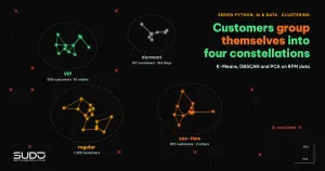
One-time buyers, regular customers and VIP customers need different messages, but nobody wants to split them up by gut feeling. Clustering solves exactly this problem: an algorithm groups similar customers on its own, with no labels to start from. This article walks through the three core clustering tools in scikit-learn, K-Means, DBSCAN and PCA, on simulated RFM (recency, frequency, monetary) data for 3,000 customers. Every number is real output from a real run.
This clustering article opens the unsupervised learning group. It follows Explaining models with SHAP: understanding why a model decides (supervised learning) and reuses the scaling knowledge from Feature engineering for tabular data: encoding, scaling and data leakage. Test environment: Apple M4, 16 GB, scikit-learn 1.9.1, NumPy 2.5.4, pandas 3.1.1.
Every API used here (KMeans, DBSCAN, PCA, silhouette_score, davies_bouldin_score, NearestNeighbors, np.random.default_rng, groupby().agg with named aggregation) has existed since scikit-learn 1.2, NumPy 1.24 and pandas 1.5, the common versions in April 2023. The data is entirely simulated.
The customer clustering problem and RFM data
For clustering, RFM analysis describes each customer with three numbers: recency is the number of days since the last purchase, frequency is the number of orders in the past 12 months, and monetary is total spend. These three numbers are enough to separate the basic shopping behaviors. In this article we generate data from four hidden groups (one-time, regular, VIP, dormant) and then hide the labels, so we can check how well the algorithm recovers the hidden structure. In practice you do not have these labels, and that is the hardest part of clustering: there is no answer key to grade against.
def seg(n, rec, freq, mon, label):
    return pd.DataFrame({
        "recency_days": rng.gamma(4, rec / 4, n).clip(1, 365),
        "frequency": rng.poisson(freq, n) + 1,
        "monetary_vnd": rng.lognormal(np.log(mon), 0.35, n),
        "true_segment": label})

df = pd.concat([seg(900, 120, 1, 400_000, "one-time"),
                seg(1400, 45, 4, 1_800_000, "regular"),
                seg(500, 12, 14, 9_000_000, "VIP"),
                seg(200, 250, 5, 2_500_000, "dormant")], ignore_index=True)
The real output of the data summary shows the scaling problem right away: monetary_vnd averages about 2.77 million with a maximum above 24 million, while frequency averages only 6 orders.
[Data] shape = (3000, 3)
      recency_days  frequency  monetary_vnd
mean          73.0        6.0     2769610.0
50%           49.0        4.0     1690528.0
max          365.0       28.0    24068896.0
K-Means: how the algorithm works
According to the scikit-learn Clustering documentation, K-Means chooses cluster centers (centroids) that minimize the inertia, the sum of squared distances from each point to its nearest center. Lloyd's algorithm repeats two steps: assign each point to the nearest center, then recompute each center as the mean of the points assigned to it. It stops when the centers move less than a tolerance. The algorithm always converges, but possibly only to a local minimum, so the documentation recommends running it several times with different initializations. The k-means++ initialization (the default) places the starting centers far apart from each other and usually gives better results than random initialization.
Because K-Means minimizes squared Euclidean distance, it implicitly assumes that clusters are convex and spherical. The documentation states plainly that inertia "responds poorly to elongated clusters or manifolds with irregular shapes", and that it does not normalize, so in high-dimensional spaces Euclidean distance inflates because of the curse of dimensionality. We will see both weaknesses in the numbers below.
Scaling before clustering
Because they rely on distances, all clustering algorithms are sensitive to scale. The first experiment in this clustering article runs K-Means with k = 4 on raw data and compares the result with the true groups using ARI (adjusted Rand index, where 1 is a perfect match and 0 is random). Next, we take the logarithm of all three columns (they are right-skewed) and standardize them with StandardScaler.
X = df.copy()
for c in X.columns:
    X[c] = np.log1p(X[c])
Xs = StandardScaler().fit_transform(X)
km = KMeans(n_clusters=4, n_init=10, random_state=0).fit(Xs)
[K-Means on raw data] ARI vs true groups = 0.481 | silhouette = 0.592
Two things stand out. First, on raw data the money column decides almost everything, so ARI is only 0.481. After log and standardization, ARI at k = 4 rises to 0.866 (see the table in the next section). Second, the silhouette on raw data (0.592) is higher than after scaling (0.457), even though the scaled clusters are far more correct. Silhouette measures separation in the very space where distances are computed, and one dominant dimension makes clusters look well separated along that dimension. Do not compare silhouette scores across two different feature spaces.
Choosing the number of clusters k
When clustering with K-Means, you must supply k. Three common internal tools are inertia (the elbow method), silhouette and Davies-Bouldin. According to the scikit-learn documentation, the silhouette coefficient of a sample is (b - a) / max(a, b), where a is the mean distance to the other points in the same cluster and b is the mean distance to the nearest other cluster. Higher values mean clearer clusters. The Davies-Bouldin index is better when lower, with a minimum of 0. We sweep k from 2 to 7 and add an ARI column (available only for simulated data) for comparison:
[Choosing k] k | inertia | silhouette | davies_bouldin | ARI
  2 |    4523.4 | 0.472 | 0.707 | 0.272
  3 |    2430.8 | 0.478 | 0.767 | 0.814
  4 |    1842.0 | 0.457 | 0.806 | 0.866
  5 |    1594.6 | 0.391 | 0.981 | 0.682
  6 |    1413.0 | 0.385 | 0.908 | 0.610
  7 |    1241.9 | 0.340 | 1.043 | 0.500
The real result is not "textbook pretty": silhouette peaks at k = 3 (0.478), Davies-Bouldin is best at k = 2 (0.707), and k = 4, the true structure of the data, ranks only second on silhouette. Inertia always drops as k grows, so the elbow shows only a bend around k = 3 to 4.
The likely cause is that the "dormant" group has only 200 customers and sits close to the "regular" group in log space, so the internal metrics prefer to merge them. Two pieces of evidence appear in the output of the cluster profile section below. At k = 3, 192 of the 200 dormant customers share a cluster with 1,356 regular customers. At k = 4, the dormant cluster's center is much closer to its nearest neighbor (1.54 standardized units) than the other clusters are (2.08 and 3.28). The right approach is to use these metrics to narrow k (3 to 5), then decide by business needs: do 200 dormant customers deserve a campaign of their own?
K-Means clustering is unstable if you skip n_init
The n_init parameter is the number of runs with different initial centers, and scikit-learn keeps the run with the lowest inertia. To see its effect, we deliberately use init="random" and run with 8 seeds:
[Stability, k=4] inertia across 8 seeds
  init=random n_init= 1: min=1842.0 max=2231.7 distinct values=3
  init=random n_init=10: min=1842.0 max=1842.0 distinct values=1
With a single initialization, one seed lands in a local minimum with an inertia of 2231.7, which is 21% worse than the best solution. With 10 initializations, all 8 seeds reach the same solution of 1842.0.
Read the profile after clustering, not just the labels
A clustering result is only valuable if the business team can name each cluster. The standard approach is to compute the median (or mean) of the original variables per cluster and keep readable units (days, orders, currency):
prof = df.assign(cluster=km.labels_).groupby("cluster").agg(
    n=("frequency", "size"), recency=("recency_days", "median"),
    frequency=("frequency", "median"), monetary=("monetary_vnd", "median"))
[Cluster profile, k=4] (median per cluster)
           n  recency  frequency   monetary
cluster
0        317    162.0        6.0  2199907.0
1       1265     39.0        5.0  1803001.0
2        913    103.0        2.0   402657.0
3        505     11.0       15.0  8891129.0
Reading the table: cluster 3 (505 customers) bought most recently, with 15 orders and nearly 8.9 million in spend: the VIP group. Cluster 1 (1,265 customers) buys steadily with moderate spend: the regular group. Cluster 2 (913 customers) buys little and spends little: one-time buyers. Cluster 0 (317 customers) once spent a fair amount but has not returned for 162 days: the win-back group. Compared with the true groups, the cross-tab shows K-Means grouped them almost correctly:
true_segment  VIP  dormant  one-time  regular
row_0
0               0      197         2      118
1               1        3         9     1252
2               0        0       889       24
3             499        0         0        6
Cluster 0 holds 197 of the 200 dormant customers but also 118 regular customers (people who have not bought in a long time and should indeed be treated as about to go dormant). To check why the internal metrics prefer k = 3, we also print the cross-tab at k = 3 and the distances between the center of cluster 0 and the other three centers:
[Cross-tab k=3: where the dormant group gets merged]
true_segment  VIP  dormant  one-time  regular
row_0
0             499        0         0       18
1               0        8       889       26
2               1      192        11     1356
[Distances from the center of cluster 0 (dormant) to the other k=4 centers, in standardized space] [1.54 2.08 3.28]
At k = 3, 192 dormant customers are merged into cluster 2 together with 1,356 regular customers, just as suspected. The distance of 1.54 to the regular cluster (cluster 1) is the smallest of the three distances.
PCA: dimensionality reduction for visualization and clustering
PCA (principal component analysis) finds the orthogonal axes along which the data varies the most. According to the scikit-learn Decomposition documentation, PCA centers the data but does not scale it before running SVD, so you must standardize first, as we did. In the context of clustering, PCA has two roles: plotting high-dimensional data on a 2D plane, and reducing noise before running K-Means (the documentation notes that PCA before K-Means "can alleviate" dimensionality problems and speed things up). Results on the RFM data:
[PCA] explained_variance_ratio_ = [0.792 0.147 0.061] | cumulative = [0.792 0.939 1.   ]
  component PC1 (recency, frequency, monetary) = [-0.538  0.591  0.601]
  K-Means on 2 PCs: silhouette = 0.514, ARI = 0.834
PC1 explains 79.2% of the variance, with a negative weight for recency and positive weights for both frequency and monetary. This is the customer "engagement" axis (bought recently, buys often, spends a lot). The first two components keep 93.9% of the variance, enough to draw a scatter plot colored by cluster. K-Means on two components gives an ARI of 0.834, slightly lower than the 0.866 with all three dimensions: dimensionality reduction always loses information, and the 6.1% of variance discarded here still carried some signal.
Does PCA rescue high-dimensional data?
Let us simulate a harder situation: add 20 columns of Gaussian noise to the standardized data (23 dimensions in total), then compare K-Means directly with K-Means after PCA down to 3 dimensions.
[Add 20 noise columns] 23 dimensions: ARI = 0.570 | PCA to 3 dimensions then K-Means: ARI = 0.565
The noise drops ARI from 0.866 to 0.570, and 3-dimensional PCA does not rescue it (0.565). The reason is that PCA keeps only the directions with large variance, and each of the 20 independent noise columns has a variance of 1, on par with many signal components, so the retained components are still mixed with noise. PCA cannot tell signal from noise; it only knows variance. For clustering, a more effective remedy is to choose business-meaningful features from the start. PCA is still very useful for visualization and for compressing highly correlated features, but do not treat it as a cure for every dimensionality problem.
DBSCAN: density-based clustering
DBSCAN (Ester, Kriegel, Sander, Xu, KDD 1996) sees clusters as high-density regions separated by low-density regions. It has two parameters: eps is the neighborhood radius, and min_samples is the minimum number of points within that radius for a point to become a core point. A cluster is a set of connected core points plus the border points near them; points that belong to no cluster get the label -1 (noise). According to the original KDD-96 paper and the sklearn.cluster.DBSCAN documentation, the advantages are that you do not need to choose the number of clusters, it finds clusters of arbitrary shape, and it has a notion of noise. The drawbacks are that eps is hard to choose, and it does poorly when clusters have very different densities.
To see the difference from K-Means, we use a two-moons dataset (1,500 points, Gaussian noise 0.07) plus 30 randomly scattered outliers:
M, ym = make_moons(1500, noise=0.07, random_state=0)
M = np.vstack([M, rng.uniform(-1.5, 2.5, (30, 2))])
kmm = KMeans(n_clusters=2, n_init=10, random_state=0).fit(M)
db = DBSCAN(eps=0.15, min_samples=8).fit(M)
[Two-moons data] K-Means vs DBSCAN
  K-Means: ARI = 0.249
  DBSCAN : ARI = 0.991 | clusters = 2 | noise points = 25
K-Means cuts the two moons in half with a straight line (ARI 0.249) because it assumes convex clusters. DBSCAN follows the shapes and finds the two clusters correctly (ARI 0.991), and it also flags 25 noise points.
Choosing eps and min_samples for DBSCAN clustering
The scikit-learn documentation stresses that eps is "very important and usually cannot be left at its default". Let us sweep eps with min_samples=8 on the two-moons data:
[DBSCAN: effect of eps, min_samples=8]
  eps=0.05: clusters=15, noise=296
  eps=0.10: clusters=2, noise=32
  eps=0.15: clusters=2, noise=25
  eps=0.30: clusters=1, noise=22
  eps=0.60: clusters=1, noise=12
Too small (0.05) and the data shatters into 15 clusters and 296 noise points; too large (0.30 and above) and the two moons stick together into one cluster. Only the narrow range of 0.10 to 0.15 gives the right answer. A systematic way to choose is to draw a k-distance graph: for each point, take the distance to its k-th neighbor (k equal to min_samples), sort the values and look for the "elbow". The k-distance percentiles on this data:
k-distance (k=8) percentiles 50/90/95/98/99: [0.048 0.082 0.102 0.146 0.633]
The distance grows slowly up to the 98th percentile (0.146) and then jumps at the 99th (0.633). That jump is the outliers, and a sensible eps sits just before the break, around 0.15. For min_samples, a common rule is at least the number of dimensions plus one, raised for noisy data.
Customer clustering with DBSCAN is genuinely harder
Applying DBSCAN to cluster the standardized three-dimensional RFM data shows its limits when clusters overlap and have different densities:
[DBSCAN on standardized 3D customer data]
  k-distance (k=10) percentiles 50/90/95/99: [0.198 0.377 0.459 0.632]
  eps=0.2: clusters=12, noise=949 (31.6%), ARI=0.135
  eps=0.3: clusters=7, noise=252 (8.4%), ARI=0.536
  eps=0.4: clusters=4, noise=67 (2.2%), ARI=0.480
  eps=0.6: clusters=2, noise=9 (0.3%), ARI=0.072
No eps gets close to the 0.866 ARI of K-Means. At eps=0.4 DBSCAN finds exactly 4 clusters, but ARI is only 0.480, because low-density VIP customers are treated as noise and adjacent groups are chained into one. Customer behavior data is usually continuous, with no clear density "valleys", so K-Means is often the first choice. DBSCAN fits better when clusters have unusual shapes (geographic coordinates, trajectories), when you need to remove noise, or for detecting anomalies, the topic of the next article.
Comparing two clustering methods: K-Means and DBSCAN
| Criterion | K-Means | DBSCAN |
|---|---|---|
| Must choose number of clusters | Yes (k) | No, but you must choose eps and min_samples |
| Cluster shape | Convex, spherical | Arbitrary |
| Noise handling | None, every point goes into a cluster | Yes, label -1 |
| Different densities | Tolerated if clusters stay convex | Poor |
| Predicting new points | Yes, predict | No predict in scikit-learn |
When not to use clustering
- You already have labels: if you have a target variable (churn, repurchase), use supervised learning. Clustering is only an exploration step and cannot replace it.
- Internal metrics are not the clustering answer: as the k-selection table above shows, silhouette and Davies-Bouldin can pick a k that differs from the business structure.
- Clustering results depend on features and scale: change the log transform or the scaling and the clusters change. Record the transformations together with the model.
- Clusters are not stable over time: customers change behavior, so you need to re-run periodically.
Common clustering mistakes
- Forgetting to scale before clustering, or forgetting to log right-skewed money variables: one column dominates, like the 0.481 ARI above.
- Stopping at numeric cluster labels without checking the cluster profile in the original units.
- Setting
n_inittoo low withinit="random", so the solution lands in a local minimum (inertia 2231.7 versus 1842.0). - Leaving DBSCAN at the default
eps(0.5) on data with a different scale: you get one giant cluster or all noise.
Checklist
- Choose features by business meaning (RFM), log-transform skewed variables, and standardize with
StandardScaler. - Before re-clustering, sweep k, check inertia, silhouette and Davies-Bouldin, then decide by business meaning.
- Use
k-means++or a large enoughn_init, and setrandom_state. - For density-based clustering with DBSCAN, draw the k-distance plot before choosing
eps, and record the noise rate. - Use PCA to visualize clustering results, along with
explained_variance_ratio_. - After every clustering run, build a cluster profile table in original units and name the clusters.
The full source is in code/s7-16 (cluster_demo.py, output.txt, requirements.txt), run with python cluster_demo.py. All numbers are real output from an Apple M4, 16 GB, scikit-learn 1.9.1 with fixed seeds; the data is simulated, and ARI can be computed only because we know the true groups.
Next article
Anomaly detection in transactions: Isolation Forest and autoencoders. DBSCAN's noise label is the simplest form of anomaly detection. The next article goes further with Isolation Forest and autoencoders, including how to evaluate when you have almost no fraud labels.