Getting a neural network to run once does not mean you know how to do deep learning training reliably. Change the learning rate from 0.001 to 0.1, with the same model and the same data, and accuracy can fall from 96% to 62%. Change the random seed and results shift by a few percent. Make a deeper network with a slightly oversized initialization and the loss turns into NaN. This article covers the four levers that decide whether deep learning training is stable: learning rate, optimizer, learning rate schedule and regularization, plus gradient clipping and early stopping. Every claim comes with a real measurement: 5 seeds, reported as mean ± standard deviation.
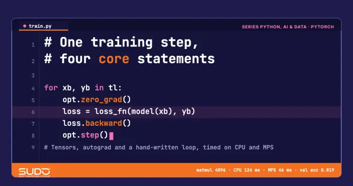
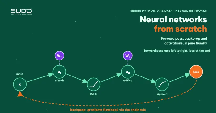
It builds on PyTorch basics: tensors, autograd and the training loop (the zero_grad, backward, step loop) and Neural networks from scratch: forward pass, backpropagation and activations. The background on gradient descent is in Linear regression and gradient descent: implementing it with NumPy; for reading test-set metrics, see Model evaluation for classifiers: precision, recall, ROC and imbalanced data. Environment: an Apple Silicon laptop with 16 GB of RAM, Python 3.12, PyTorch, scikit-learn and NumPy, running on CPU. The APIs used here (AdamW, OneCycleLR, LambdaLR, clip_grad_norm_) have existed since PyTorch 1.x and work the same way in the 2.x line.
Setting up a reproducible deep learning training experiment
To compare ways of doing deep learning training, you have to remove noise first. We use scikit-learn's 8x8 handwritten digits dataset (1,797 images, 10 classes): 600 images to train the model, 598 for validation and 599 for the final test. The test set is not used to choose any hyperparameter in this article. The model is an MLP with two hidden layers of 256 units; each configuration runs with seeds 0 to 4, and every run resets random, NumPy and PyTorch.
def set_seed(seed: int) -> None:
    random.seed(seed)
    np.random.seed(seed)
    torch.manual_seed(seed)

# shuffle data with a dedicated generator so mini-batch order is repeatable
g = torch.Generator().manual_seed(seed)
perm = torch.randperm(len(X_tr), generator=g)
train/val/test = [600, 598, 599]With 598 validation samples, one sample changing its label shifts accuracy by about 0.17 percentage points. So when two configurations differ by less than one standard deviation, we call it a tie and draw no conclusion. This is basic discipline in deep learning training: reporting a single run is reporting noise.
Learning rate in deep learning training: the most important hyperparameter
The learning rate (lr) is the length of each weight update step. In deep learning training, an lr that is too small makes the loss fall so slowly it looks like nothing is learning; one that is too large overshoots the bottom of the valley, and the loss oscillates or diverges. We sweep lr over powers of 10 with Adam for 30 epochs:
lr=1e-05   val_acc=0.666 ± 0.054  val_loss=2.173 ± 0.005
lr=0.0001  val_acc=0.916 ± 0.002  val_loss=0.397 ± 0.003
lr=0.001   val_acc=0.963 ± 0.002  val_loss=0.146 ± 0.005
lr=0.01    val_acc=0.961 ± 0.009  val_loss=0.182 ± 0.057
lr=0.1     val_acc=0.618 ± 0.175  val_loss=1.230 ± 0.276
In deep learning training, this inverted-U shape shows up in most problems: there is a wide band of lr (here 1e-3 to 1e-2) with similar results, and two different failure modes on either side. At 1e-5, a val_loss of 2.173 is close to ln(10) = 2.303, meaning the model has barely moved off a uniform guess over 10 classes. At 0.1, the standard deviation jumps to 0.175: the result depends on the seed, a clear sign of unstable deep learning training. The practical procedure for deep learning training is to run a few dozen steps at several learning rates, pick the largest lr at which the loss still falls smoothly, then back off a little. There is no "right" lr for every model, because the best value depends on the optimizer, the batch size and the architecture.
Optimizers for deep learning training: SGD, momentum, Adam and AdamW
SGD updates w -= lr * grad on each mini-batch. Momentum accumulates a moving average of the gradient, which helps it cross flat regions and reduces oscillation. Adam (Kingma and Ba, ICLR 2015, the original paper on arXiv) estimates both the first and second moments of the gradient so each parameter gets its own step size, which makes it less sensitive to gradient scale than SGD. Compared under identical conditions (30 epochs):
SGD lr=0.01                val_acc=0.780 ± 0.025  val_loss=1.795 ± 0.035
SGD lr=0.1                 val_acc=0.946 ± 0.004  val_loss=0.192 ± 0.006
SGD+momentum 0.9 lr=0.05   val_acc=0.966 ± 0.002  val_loss=0.157 ± 0.005
Adam lr=1e-3               val_acc=0.963 ± 0.002  val_loss=0.146 ± 0.005
AdamW lr=1e-3 wd=0.01      val_acc=0.963 ± 0.003  val_loss=0.146 ± 0.006
Two lessons for deep learning training. First, plain SGD is very sensitive to lr: going from 0.01 to 0.1 raises accuracy from 0.780 to 0.946 with the same number of epochs, so "SGD is bad" often just means "the lr is wrong". Second, on this small problem, SGD with momentum, Adam and AdamW all land within the same noise band (0.963 to 0.966). Do not conclude that "all optimizers are the same" for large models; conclude instead that the gap between good optimizers is usually smaller than the gap caused by a wrong lr.
AdamW: weight decay decoupled from the gradient
In torch.optim.Adam, the weight_decay parameter adds wd * w to the gradient (that is, L2 regularization) before passing it through Adam's adaptive normalization. Loshchilov and Hutter show in Decoupled Weight Decay Regularization that for adaptive optimizers, L2 and weight decay are not equivalent. AdamW fixes this by shrinking the weights directly: w <- w * (1 - lr * wd), without going through the gradient. We verify it with a loss that has no gradient, leaving only the decay term:
Adam  (L2)         wd=0.01  w after 100 steps: 0.90174
Adam  (L2)         wd=0.1   w after 100 steps: 0.90174
AdamW (decoupled)  wd=0.01  w after 100 steps: 0.99900
AdamW (decoupled)  wd=0.1   w after 100 steps: 0.99005
AdamW formula: (1 - 1e-3*0.01)^100 = 0.99900; (1 - 1e-3*0.1)^100 = 0.99005
An interesting result: with Adam, wd=0.01 and wd=0.1 give the same answer, 0.90174. The gradient consists only of the L2 term, and Adam divides the gradient by the square root of the second moment, so the magnitude of wd cancels out and every step moves by about lr. With AdamW, the weights shrink exactly as (1 - lr*wd)^steps and wd really controls the strength. This is why AdamW is the default choice when you need weight decay with large models. Note that torch.optim.AdamW defaults to weight_decay=0.01, while Adam defaults to 0.
Learning rate schedule in deep learning training: warmup and cosine
Holding lr constant in deep learning training is simple but wasteful: early on, large steps make fast progress; late in training, small steps settle into the bottom. Two common components are warmup (raising lr from a small value over the first few epochs, so updates do not wreck the weights while Adam's moments are still unstable) and cosine annealing (decreasing lr along half a cosine curve to 0, an idea from SGDR by Loshchilov and Hutter). We implement the multiplier with LambdaLR and compare it with PyTorch's built-in OneCycleLR:
def warmup_cosine(step, total, warmup):
    if step < warmup:
        return (step + 1) / warmup
    p = (step - warmup) / max(1, total - warmup)
    return 0.5 * (1 + math.cos(math.pi * p))

opt = torch.optim.Adam(model.parameters(), lr=3e-3)
sched = torch.optim.lr_scheduler.LambdaLR(opt, lambda s: warmup_cosine(s, total, warmup=3 * steps_per_epoch))
# in the loop: opt.step() first, then sched.step(), once per mini-batch
Calling optimizer.step() before scheduler.step() is the PyTorch convention; reversing them skips the first lr value and PyTorch emits a warning. The lr values logged after epochs 1, 11, 21, 31, 41 and 51 (from lr_samples_output.txt) show the shape of the three schedules:
{"const":    [0.003, 0.003, 0.003, 0.003, 0.003, 0.003],
 "cosine":   [0.00105, 0.00286, 0.00232, 0.00154, 0.00075, 0.00018],
 "onecycle": [0.00014, 0.00206, 0.00296, 0.00234, 0.00127, 0.00032]}
Results after 60 epochs, 5 seeds:
constant         val_acc=0.964 ± 0.002 val_loss=0.158 ± 0.004
warmup + cosine  val_acc=0.965 ± 0.004 val_loss=0.143 ± 0.005
OneCycleLR       val_acc=0.962 ± 0.002 val_loss=0.143 ± 0.005
Accuracy is a tie (0.962 to 0.965), but val_loss drops from 0.158 to 0.143 with both decaying schedules, beyond the noise (standard deviation 0.004 to 0.005). The explanation: when lr approaches 0 at the end of training, the weights stop bouncing around the bottom, so the output probabilities become more stable. For this small model the benefit is modest; for deep networks with large batches, warmup can decide whether the model learns at all.
When using OneCycleLR for deep learning training, note that it differs from our hand-written version in two ways: by default it also cycles momentum (for Adam, beta1 moves between 0.85 and 0.95, opposite to lr, controlled by cycle_momentum), and it uses one long ramp-up phase (30% of the steps by default) followed by cosine decay, so it is not a 3-epoch warmup like the one above. Besides these two schedules, StepLR, ReduceLROnPlateau (lowers lr when val_loss stops improving) and CosineAnnealingWarmRestarts are also available in torch.optim.lr_scheduler; see the torch.optim documentation.
Regularization in deep learning training: dropout, weight decay and overfitting
To see overfitting in deep learning training, we increase model capacity (512 units per layer) and run 100 epochs with AdamW at lr=1e-3. The model reaches a train accuracy of 1.000 in every configuration, so what we compare is val_loss, the amount of confident error on unseen samples:
no regularization      train_acc=1.000 ± 0.000 val_acc=0.962 ± 0.001 final val_loss=0.152 ± 0.007 min val_loss=0.128 ± 0.006
weight decay 0.1       train_acc=1.000 ± 0.000 val_acc=0.964 ± 0.003 final val_loss=0.132 ± 0.005 min val_loss=0.126 ± 0.005
dropout 0.3            train_acc=1.000 ± 0.000 val_acc=0.972 ± 0.005 final val_loss=0.128 ± 0.014 min val_loss=0.110 ± 0.003
dropout 0.3 + wd 0.1   train_acc=1.000 ± 0.000 val_acc=0.971 ± 0.003 final val_loss=0.117 ± 0.009 min val_loss=0.103 ± 0.004
The last two columns say something important for deep learning training: without regularization, the lowest val_loss is 0.128 but the final one is 0.152, so the model was better in the middle of training and then got worse through overfitting. Dropout at 0.3 (randomly turning off 30% of units during training; model.eval() turns it off during evaluation) lifts val_acc to 0.972; combining it with weight decay 0.1 gives the lowest final val_loss (0.117). For deep learning training at this scale, the accuracy gain is about one percentage point, just large enough to exceed the standard deviation, but it is still a small dataset: do not copy the numbers, copy the method.
Early stopping: stop when validation stops improving
In deep learning training, the cheapest way to recover the "best in the middle of training" point is early stopping: watch val_loss, and if it has not improved after patience epochs, stop and reload the best weights.
if vl < best - 1e-4:
    best, bad = vl, 0
    best_state = {k: v.clone() for k, v in model.state_dict().items()}
else:
    bad += 1
    if bad >= patience:
        break
model.load_state_dict(best_state)
run all 100 epochs : val_acc=0.962 ± 0.001 val_loss=0.152 ± 0.007
early stopping : val_acc=0.969 ± 0.002 val_loss=0.128 ± 0.007
best epoch / stop epoch per seed: [(17, 25), (19, 27), (20, 28), (25, 33), (18, 26)]With patience=8, training stops at epochs 25 to 33 instead of 100, saving about 70% of the time while val_loss is better (0.128 versus 0.152). A subtle point: we pick the epoch using the validation set, so the early-stopping val_acc is slightly optimistic; the final number must be reported on the test set, which we have not touched yet. We touch it exactly once in the whole deep learning training process of this article, for the final configuration chosen from the sections above (AdamW lr=1e-3, weight decay 0.1, dropout 0.3, warmup plus cosine, early stopping), run with final_test.py over 5 seeds:
AdamW lr=1e-3 wd=0.1 dropout=0.3 hidden=512, warmup+cosine, early stopping patience=8
val_acc  = 0.970 ± 0.002
test_acc = 0.971 ± 0.002  (599 samples, run once)
test_loss= 0.130 ± 0.006
best epoch per seed: [24, 47, 45, 44, 26]
Test accuracy (0.971) is very close to validation (0.970), so choosing the configuration on validation did not make the numbers noticeably optimistic on this small problem. This figure is a single measurement of the deep learning training procedure and is not used to tune any further hyperparameter.
Gradient clipping: keeping deep learning training from blowing up
In deep learning training, gradient clipping limits the total magnitude of the gradient before the update. torch.nn.utils.clip_grad_norm_(parameters, max_norm) computes the L2 norm of all gradients, multiplies them all by max_norm / norm if the norm exceeds max_norm, and returns the norm before clipping, which is handy for logging. It must be called after backward() and before step(). To create controlled instability, we use an 8-layer MLP with weights initialized as std = gain / sqrt(fan_in) and SGD at lr=0.05. For ReLU, He (Kaiming) initialization uses gain = sqrt(2) ≈ 1.41 (see torch.nn.init.calculate_gain), so a gain of 1.5 is close to the standard and a gain of 2.0 is far too large:
gn = torch.nn.utils.clip_grad_norm_(model.parameters(), max_norm=1.0)
opt.step()
gain=1.5 lr=0.05 clip=None: final val_acc=0.954 ± 0.008 loss=NaN: 0/5 max gradient norm=16.1
gain=1.5 lr=0.05 clip=1.0: final val_acc=0.919 ± 0.015 loss=NaN: 0/5 max gradient norm=16.2
gain=2.0 lr=0.05 clip=None: final val_acc=0.432 ± 0.406 loss=NaN: 3/5 max gradient norm=inf
gain=2.0 lr=0.05 clip=1.0: final val_acc=0.877 ± 0.011 loss=NaN: 0/5 max gradient norm=241The result cuts both ways in deep learning training, and both sides are worth remembering. When learning is already stable (gain 1.5, close to He), clipping the gradient at 1.0 hurts: accuracy falls from 0.954 to 0.919 because normal gradients are already larger than 1, so every step gets shrunk. When the initialization is too large (gain 2.0), no clipping leaves 3 of 5 runs ending in NaN (the gradient norm reaches infinity), while with clipping all 5 runs converge to 0.877 ± 0.011. The practical conclusion: clipping is a safety net, not a tonic. Log the gradient norm first, set max_norm above the typical norm (for example the 90th to 99th percentile), and turn it on only when you see spikes.
How major frameworks set their defaults
| Component | Common default | Notes |
|---|---|---|
| Optimizer | AdamW, lr 1e-4 to 1e-3 | Very common for Transformers and fine-tuning; SGD+momentum is still common for vision CNNs |
| Weight decay | 0.01 to 0.1 with AdamW | Usually not applied to biases and normalization parameters |
| Schedule | Linear warmup + cosine, or linear decay to 0 | Warmup of a few hundred to a few thousand steps for large models |
| Gradient clipping | max_norm=1.0 | Common in deep learning training of Transformers; verify against the gradient norm log |
| Early stopping | patience 3 to 10 epochs | Choose by val_loss rather than val_acc because it is smoother |
The defaults above are widely used starting points, not rules. Any conclusion we draw has to come from experiments on our own data.
When not to overcomplicate deep learning training
- Tabular data: gradient boosting usually beats neural networks without needing most of the tuning in this article (see Gradient boosting with XGBoost and LightGBM: when it beats deep learning).
- Very little data: instead of tuning lr for a model trained from scratch, use a pretrained model (next article).
- No baseline yet: if you have not compared against logistic regression or a simple model, any optimizer tuning is premature.
Common mistakes in deep learning training
- Forgetting
model.train()andmodel.eval(): dropout and batch norm behave differently in the two modes; forgettingeval()during evaluation makes val_loss jump around. - Calling
scheduler.step()at the wrong interval: a schedule defined per mini-batch but stepped per epoch (or the reverse) gives lr the wrong shape; printopt.param_groups[0]["lr"]. - Choosing hyperparameters on the test set: leads to overly optimistic final numbers. Choose on validation, report on test once.
- Running a single seed in deep learning training: a difference of 0.3 percentage points is usually noise; use at least 3 to 5 seeds.
- Using
weight_decayin Adam as if it were AdamW: they are different things, as measured above. - Clipping too aggressively: a
max_normbelow the typical gradient norm slows training, as the gain 1.5 result shows. - Not logging the gradient norm and lr: without those numbers you cannot diagnose why the loss diverges.
Checklist for stable deep learning training
- For deep learning training, fix the seeds, run at least 3 seeds and report mean ± standard deviation.
- Sweep lr over powers of 10 first, and only then tune other things.
- Start with AdamW; try SGD+momentum for vision CNNs.
- Use warmup + cosine; record the actual lr at every epoch.
- Watch val_loss (not just val_acc); use early stopping and keep the best weights.
- Add dropout and weight decay when train accuracy hits 100% and val_loss starts to rise.
- Log the gradient norm; turn clipping on only when you see spikes.
All the code is in code/s7-22 (train_lib.py, experiments.py, adam_vs_adamw.py, final_test.py, the output files and requirements.txt, which does not pin versions); run it with python experiments.py. The recorded run took 221 seconds on a 16 GB laptop CPU while the machine was busy with other tasks, with peak memory around 340 MB (measured with /usr/bin/time -l, saved in time_experiments.txt). Every deep learning training number in this article is real output from that run. The data is a small handwritten-digits set, so do not carry the absolute numbers over to another problem.
Next article
Image classification with CNNs and transfer learning in PyTorch. When you only have a few hundred images, deep learning training from scratch fails even after tuning everything in this article. The next article uses a ResNet18 pretrained on ImageNet and measures the difference between freezing, fine-tuning and learning from scratch.