In earlier articles we wrote gradient descent by hand with NumPy: derivatives worked out on paper, updates applied manually. That approach teaches the fundamentals, but it breaks down once a model has thousands of parameters and many layers. PyTorch solves exactly that with three pieces: tensors (multidimensional arrays that run on CPU and GPU), autograd (automatic differentiation) and torch.nn (the building blocks for models). This article goes from PyTorch tensors to autograd, then to a complete training loop with nn.Module, DataLoader and Adam, with real output at every step.
It continues Building a product recommender in Python: content-based and collaborative filtering, where we implemented ALS ourselves in NumPy. Linear regression and gradient descent: implementing it with NumPy is the direct foundation for the training-loop section, and a tensor is essentially an upgraded NumPy array, so revisit NumPy for machine learning: vectorization and broadcasting if needed. Environment: a Mac with an Apple Silicon chip, 16 GB of RAM, Python 3 and the latest stable PyTorch at the time of running; every API used here has existed since PyTorch 2.0 (released in March 2023) or earlier. All data is synthetic.
PyTorch tensors: like NumPy, plus what extra
According to the PyTorch Tensors tutorial, a tensor is the core data structure, similar to a NumPy array but able to run on GPUs and other accelerators. Three attributes to remember are shape, dtype and device; a new tensor lives on the CPU by default.
a = torch.tensor([[1.0, 2.0, 3.0], [4.0, 5.0, 6.0]])
b = torch.tensor([10.0, 20.0, 30.0])
print(a + b)       # broadcasting, as in NumPy
print(a @ a.T)     # matrix multiplication
MPS: True
[1. Tensor]
a.shape = (2, 3) | dtype = torch.float32 | device = cpu
int tensor dtype: torch.int64
broadcasting a + b =
tensor([[11., 22., 33.],
[14., 25., 36.]])
a @ a.T =
tensor([[14., 32.],
[32., 77.]])Two differences from NumPy are worth noting when you start using PyTorch. First, floating-point numbers default to float32 (NumPy uses float64), because neural networks do not need double precision and float32 is faster and uses less memory. Second, dtype is strict: multiplying a float tensor by an integer tensor raises an error instead of silently casting, as we will see in the common-mistakes section.
The bridge between PyTorch and NumPy is also worth understanding. The documentation says that a CPU tensor and a NumPy array can share memory. We can check this by creating two tensors from the same array and then modifying the original array:
n = np.array([1.0, 2.0, 3.0])
t = torch.from_numpy(n)       # shares memory with n
t2 = torch.tensor(n)          # torch.tensor always copies
n[0] = 99.0
after modifying n[0] = 99: from_numpy t = [99.0, 2.0, 3.0] | torch.tensor t2 = [1.0, 2.0, 3.0]from_numpy sees the change because it does not copy; torch.tensor copies, so it is unaffected. A classic mistake is changing the original NumPy data and forgetting that a tensor points at the same memory. The documentation also advises avoiding in-place operations (names with a trailing underscore such as add_), because they save memory but can cause trouble when computing gradients.
PyTorch autograd: computing derivatives automatically
In PyTorch, according to the Automatic Differentiation with torch.autograd tutorial, tensors that need gradients (such as model parameters) are marked with requires_grad=True. Every operation on them is recorded as a Function node in the computation graph; the grad_fn attribute of each tensor points to the backward function that produced it. Calling loss.backward() walks the graph in reverse and fills in the .grad of the leaf tensors.
x = torch.tensor(3.0, requires_grad=True)
y = x ** 2 + 2 * x + 1        # y = (x+1)^2, dy/dx = 2x + 2
y.backward()
print(x.grad)                 # 8.0
[2. Autograd]
y = 16.0 | y.grad_fn = <AddBackward0 object at 0x10e8c7e80>
dy/dx at x=3: 8.0 (analytic: 2*3+2 = 8)The result 8.0 matches the analytic formula 2x + 2 at x = 3. The important point is that, as the documentation explains, this graph is a DAG rebuilt from scratch after every backward() call; that is why a model can use if statements, loops and changing shapes between runs. This is why PyTorch is called "define-by-run": we write ordinary Python, and the graph is built as the code executes.
Gradient accumulation in PyTorch: why you must call zero_grad
The same documentation points out that successive backward() calls add to .grad rather than overwrite it. We can verify this by running backward twice on the same variable:
second backward without zeroing: x.grad = 16.0 (accumulated: 8 + 8)
after zero_(): 0.0
The correct derivative is still 8, but .grad becomes 16. In a training loop, if you forget to clear it, the gradients of successive batches pile up and the update step goes in the wrong direction with the wrong size. We measured the consequence on a small linear regression (same data, same learning rate of 0.1, 30 SGD steps):
[4. Forgetting zero_grad]
with zero_grad   : loss after 30 steps = 0.0116
without zero_grad: loss after 30 steps = 8.388
Same model, same data: a loss of 0.0116 versus 8.388, just because one line is missing. It is also a silent bug, since the program reports nothing and the loss merely looks "strange". There are two ways to stop gradients from being tracked when you do not need them: torch.no_grad() turns off graph recording for the whole block, while detach() returns a tensor separated from the graph.
inside no_grad: z.requires_grad = False
detach(): requires_grad = False
Checking autograd with a numerical derivative
When you write a new operation yourself, the most trustworthy check is to compare the autograd gradient with the central difference (f(w+e) - f(w-e)) / 2e. We try it on a squared loss over a dot product:
w = torch.tensor([1.0, -2.0], requires_grad=True)
xx = torch.tensor([3.0, 4.0])
loss = ((w * xx).sum() - 5.0) ** 2
loss.backward()
autograd gradient : [-60.0, -80.0]
numerical gradient (finite difference): [-60.005, -79.994]The two results agree up to the error of the finite difference, as expected: loss = (3w0 + 4w1 - 5)^2 has derivatives 2(3w0 + 4w1 - 5) times 3 and 4, which is -60 and -80 at this point. PyTorch ships torch.autograd.gradcheck, which does exactly this for a custom function.
A hand-written PyTorch training loop
Putting the PyTorch pieces together: forward pass to get predictions, compute the loss, backward() to get gradients, update the parameters, clear the gradients. We redo linear regression with three features, but the gradients now come from autograd instead of a hand-written formula, and the update sits inside torch.no_grad() so that subtracting the gradient is not recorded in the graph.
# X, y: 200 samples, 3 features, generated in pytorch_basics.py (y = X @ [2, -1, 0.5] + 4 + noise)
w = torch.zeros(3, requires_grad=True); b = torch.zeros(1, requires_grad=True)
lr = 0.1
for epoch in range(101):
    pred = X @ w + b
    loss = ((pred - y) ** 2).mean()
    loss.backward()
    with torch.no_grad():
        w -= lr * w.grad
        b -= lr * b.grad
    w.grad.zero_(); b.grad.zero_()
[3. Linear regression, manual update]
epoch 0 loss = 21.42914
epoch 25 loss = 0.01250
epoch 50 loss = 0.01138
epoch 75 loss = 0.01138
epoch 100 loss = 0.01138
learned w: [1.994, -1.003, 0.495] | b: 4.0 | true: [2.0, -1.0, 0.5], 4.0
least-squares solution: [1.994, -1.003, 0.495, 4.0]The data is generated with true weights (2, -1, 0.5), an intercept of 4 and noise of 0.1. The model learns (1.994, -1.003, 0.495; 4.0), matching to three digits the least-squares solution computed directly with torch.linalg.lstsq. The loss settles at 0.01138, roughly the noise variance of 0.1 squared, which is the lowest value possible. The result is the same kind as in the NumPy gradient descent article, but this time we wrote no derivative at all; PyTorch took care of that.
PyTorch nn.Module, DataLoader and optimizer
Writing every parameter by hand is only fine for small models. According to the Optimizing Model Parameters tutorial, each training pass over a batch consists of: forward (pred = model(X), loss = loss_fn(pred, y)), loss.backward(), optimizer.step(), then optimizer.zero_grad(). The tutorial also names three basic hyperparameters: the number of epochs, the batch size and the learning rate; model.train() and model.eval() set the mode for layers such as dropout and batch normalization, and torch.no_grad() wraps evaluation to skip gradient computation.
We apply this to a binary classification problem on 4,000 synthetic customers with 6 features, where the labels are generated from a nonlinear function (including a product term of two features). We split 3,000 for training and 1,000 for validation. The network has one hidden layer of 16 neurons with ReLU:
# tl: DataLoader over the 3,000 training samples, created in pytorch_basics.py
class Net(nn.Module):
    def __init__(self):
        super().__init__()
        self.body = nn.Sequential(nn.Linear(6, 16), nn.ReLU(), nn.Linear(16, 1))
    def forward(self, x):
        return self.body(x).squeeze(1)

model = Net()
loss_fn = nn.BCEWithLogitsLoss()
opt = torch.optim.Adam(model.parameters(), lr=1e-2)

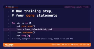
for epoch in range(1, 21):
    model.train()
    for xb, yb in tl:                 # tl = DataLoader(batch_size=64, shuffle=True)
        opt.zero_grad()
        loss = loss_fn(model(xb), yb)
        loss.backward()
        opt.step()
Two design details of PyTorch here. First, the last layer has no sigmoid, because BCEWithLogitsLoss combines the sigmoid with cross-entropy in a more numerically stable way; the positive class is predicted when the logit is greater than 0. Second, DataLoader handles batching and shuffling, so the loop is left with only four core statements (zero_grad, computing the loss from the forward pass, backward, step).
[5. Classification with nn.Module, DataLoader, Adam]
positive label rate: 0.563
number of parameters: 129
majority-class baseline on validation: acc = 0.558
epoch  1 | val loss 0.4398 | val acc 0.794
epoch  5 | val loss 0.3975 | val acc 0.823
epoch 10 | val loss 0.4008 | val acc 0.814
epoch 20 | val loss 0.3989 | val acc 0.819
training time for 20 epochs on CPU: 0.31s
The PyTorch network with 129 parameters reaches 0.819 validation accuracy versus 0.558 for the majority-class baseline, taking about 0.31 seconds for 20 epochs on CPU. The more important observation than the number: validation loss falls from 0.4398 to 0.3975 by epoch 5 and then hovers around 0.40; the model has learned all the signal this small architecture can capture, and training longer does not help. Watching validation loss like this will be the basis for the training-stability article later in the series.
Finally, saving and loading. The recommended approach is to save the state_dict (the dictionary of parameters) rather than the whole model object, and to load it with torch.load(..., weights_only=True) so that no arbitrary code in the pickle file gets executed:
save and load state_dict, predictions match: TruePyTorch on CPU or MPS: when a GPU is worth it
A PyTorch tensor can be moved to another device with .to(device); on a Mac with an Apple Silicon chip, the GPU backend is called mps. We timed the multiplication of two square matrices, averaged over 20 runs, after 3 warm-up runs and with a synchronize before starting the timer (GPUs run asynchronously, so timing without synchronizing gives wrong results):
[6. CPU vs MPS (Mac with Apple Silicon chip)]
matmul   64x64    CPU    0.002 ms | MPS    0.083 ms
matmul 1024x1024  CPU    1.523 ms | MPS    1.404 ms
matmul 4096x4096  CPU  124.344 ms | MPS   46.415 ms
Across three consecutive runs (all recorded in output.txt), the 4096x4096 matrix took 109 to 124 ms on CPU and 43 to 46 ms on MPS; the 1024x1024 matrix showed a modest difference. For the small 64x64 matrix, MPS is many times slower than CPU because launch and communication overhead outweigh the computation. The lesson: a GPU is worth using only when each call carries enough work. The 129-parameter network above running on CPU with PyTorch is reasonable; moving to MPS or an NVIDIA GPU only makes sense when the model and batch are large enough. These are measurements from one machine, not a general conclusion for all hardware, and do not forget that copying large tensors between devices also takes time.
When not to use PyTorch
PyTorch is powerful, but it is not always the right tool, and you should think twice before pulling it into a project:
- Small tabular datasets: as in the article on gradient boosting with XGBoost and LightGBM, boosted trees often beat neural networks and are much simpler. The network above should be treated only as a textbook example.
- Linear models, trees and classic clustering: scikit-learn already provides them, with Pipeline and cross-validation, as in Machine learning with scikit-learn: Pipeline, cross-validation and tuning.
- When every decision must be explainable: neural networks are harder to explain and need tools such as SHAP alongside them.
- Constrained runtime environments: PyTorch is a heavy library (a virtual environment with torch and numpy installed takes 786 MB according to
du -sh, recorded inoutput.txt) and is hard to fit into a small container; when serving a model, it is usually exported to a more compact format.
Common PyTorch mistakes
- Forgetting
zero_grad(): gradients accumulate, giving a loss of 8.388 instead of 0.0116 as measured above. - dtype mismatch: multiplying a float by an integer gives a clear error. Real output:
dot : expected both vectors to have same dtype, but found Float and Long. Labels forBCEWithLogitsLossmust be float, while labels forCrossEntropyLossare integers (long). - In-place edits of leaf parameters:
w.add_(1.0)on a tensor that requires gradients raisesa leaf Variable that requires grad is being used in an in-place operation. To update a parameter, do it insidetorch.no_grad(), as in the hand-written loop. - Forgetting
model.eval()during evaluation: dropout and batch norm stay in training mode, so evaluation results are noisy and not reproducible. - Forgetting
no_grad()during inference: it wastes memory because the graph is still recorded. - Not setting a seed: results change from run to run; use
torch.manual_seed. Even with a seed, PyTorch results can differ between CPU and GPU. - Timing a GPU without synchronizing: not calling
torch.mps.synchronize()(or the CUDA equivalent) before starting the timer gives wrong measurements.
PyTorch basics checklist
- PyTorch tensors default to float32; check
shape,dtypeanddevicewhen you hit an error. from_numpyshares memory,torch.tensorcopies.requires_grad=Truefor parameters;backward()fills.grad; gradients accumulate.- The standard loop:
zero_grad(), forward, loss,backward(),step(). - Evaluate a PyTorch model under
model.eval()andtorch.no_grad(); watch validation loss, not just train loss. - Save the
state_dict, load withweights_only=True. - Validate a PyTorch model against a baseline and a numerical derivative; use a GPU only when each call is large enough.
The full source is in code/s7-20 (pytorch_basics.py, output.txt, requirements.txt, versions not pinned), run with python pytorch_basics.py. All PyTorch figures in this article are real output from a Mac with an Apple Silicon chip and 16 GB of RAM; timings vary slightly between runs, while loss and accuracy values are fixed by the seed; the data is synthetic.
Next article
Neural networks from scratch: forward pass, backpropagation and activations. Autograd does everything in a single backward() line; the next article opens up that black box by implementing a neural network and backpropagation ourselves in NumPy, then comparing the result with PyTorch.