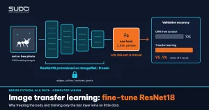
You have 244 training images, two classes (ants and bees), and you want an image classifier. Training a CNN from scratch gives 71.9% on the validation set (153 images: 70 ants, 83 bees, so always guessing "bee" already scores 54.2%). But if you take a network that has already learned from millions of ImageNet images, keep the entire feature extractor frozen and train only the 1,026 parameters of the last layer, accuracy rises to 95.9%.
That is the power of transfer learning: reusing visual knowledge learned on a large problem to solve your small one. This article explains why it works, how to implement it correctly with PyTorch and torchvision, and the practical traps, with real measurements averaged over 3 seeds on an Apple Silicon machine.
It builds on Stable deep learning training: optimizers, learning rates and regularization (learning rate, schedules, overfitting) and PyTorch basics: tensors, autograd and the training loop. For how to read accuracy and pick a metric, see Model evaluation for classifiers: precision, recall, ROC and imbalanced data. Environment: Apple Silicon, 16 GB, Metal GPU (device="mps"), Python 3.10, PyTorch 2.1.1, torchvision 0.16.1. The torchvision weights= API has existed since version 0.13 (2022), so the code works with 0.13 and later.
CNNs and why transfer learning works
A convolutional neural network (CNN) processes images with small filters that slide across the image. The first layers learn simple patterns such as edges and colors; the middle layers combine them into corners, textures and parts; the last layers recognize whole objects. The paper How transferable are features in deep neural networks? by Yosinski et al. (NeurIPS 2014) measured exactly this: early layers are general, later layers become increasingly specific to the original task, and initializing with transferred features beats random initialization even after fine-tuning. That is the basis of transfer learning for images: the early part of a network trained on ImageNet is still useful for photos of bees and ants.
The network we use is ResNet18, from the ResNet family by He et al. (Deep Residual Learning for Image Recognition, 2015), where each block learns a residual relative to its input through a skip connection, which makes deep networks trainable. According to the table in the torchvision models documentation, the IMAGENET1K_V1 weights of ResNet18 reach 69.758% top-1 on ImageNet-1K with 11.7 million parameters. It is a small model that runs well on a laptop, so it suits a transfer learning demo.
| Strategy | Trained parameters | When it fits |
|---|---|---|
| Train from scratch | All, randomly initialized | Very large dataset, images very different from ImageNet (medical, satellite) |
| Feature extractor (frozen) | Only the new classifier layer | Very little data, images close to natural photos |
| Full fine-tuning | All, initialized from ImageNet, small lr | A moderate amount of data, higher accuracy needed |
The two transfer learning scenarios, freezing and fine-tuning, are the same two scenarios as in the official PyTorch Transfer Learning tutorial, which uses the same ants/bees dataset. We reuse that dataset so readers can compare results, but we write the code and take the measurements ourselves.
Data preparation and preprocessing for transfer learning
The hymenoptera_data dataset is a very small subset of ImageNet, provided by the PyTorch documentation for learning; under the ImageNet terms it is for research and educational use only. Its folder structure train/ants, train/bees, val/ants, val/bees matches torchvision.datasets.ImageFolder.
torch 2.1.1 | torchvision 0.16.1 | device mps
train 244 val 153 classes ['ants', 'bees']
With 153 validation images, a single changed prediction moves accuracy by 0.65 percentage points, so differences smaller than about 1 point are not trustworthy. The most important rule when preparing data for transfer learning is to use exactly the preprocessing the original network was trained with: resize to 256, center crop to 224, scale to [0,1], then normalize with the ImageNet mean/std. Torchvision bundles this together with the weights:
w = models.ResNet18_Weights.IMAGENET1K_V1
m = models.resnet18(weights=w).eval()
prep = w.transforms()
print(prep)
print(w.meta["_metrics"]["ImageNet-1K"]["acc@1"], w.meta["num_params"])
Note: _metrics is an internal metadata key in torchvision (it has a leading underscore), not a public API, so it may change in a later release; if you need this number for a report, check it against the table in the documentation.
ImageClassification(
    crop_size=[224]
    resize_size=[256]
    mean=[0.485, 0.456, 0.406]
    std=[0.229, 0.224, 0.225]
    interpolation=InterpolationMode.BILINEAR
)
published acc@1: 69.758 | parameters: 11689512
Note how we write it: we pass IMAGENET1K_V1 explicitly instead of weights="DEFAULT", because the documentation warns that the DEFAULT alias may point to a different set of weights in a later version, making results unrepeatable. The old pretrained=True argument has been deprecated since version 0.13. Running the original model on the first two images of the validation set shows that it still speaks in the 1,000 ImageNet classes:
ants/10308379_1b6c72e180.jpg: fountain 0.12, shovel 0.08, snowplow 0.04
bees/1032546534_06907fe3b3.jpg: apiary 0.48, bee 0.27, honeycomb 0.25
These are two single images, not statistics, but they clearly show that the original output does not give us the labels "ant, bee"; we need to replace the last layer and train that part again. For the training set only, we add data augmentation: RandomResizedCrop(224, scale=(0.5, 1.0)) and RandomHorizontalFlip(), so the model sees each image in many forms every epoch.
Implementing transfer learning in PyTorch: replace the head, freeze the body
Every torchvision model has a final classification layer; for ResNet18 it is m.fc, which takes a 512-dimensional vector. The standard procedure has three steps: load the weights, optionally freeze, and replace the last layer with a new one whose output size matches your problem.
def resnet(mode):
    m = models.resnet18(weights=weights)
    in_f = m.fc.in_features
    if mode == "freeze":
        for p in m.parameters():
            p.requires_grad = False   # freeze the whole network body
    m.fc = nn.Linear(in_f, 2)         # new layer: requires_grad=True by default
    return m
The order is critical: replace fc after freezing, because the newly created layer has requires_grad=True. If you do it the other way around, you freeze the new layer as well and there is nothing left to learn. Verify the transfer learning setup by counting parameters:
python transfer.py params
mode freeze: trainable 1,026 / total 11,177,538 parameters
mode full: trainable 11,177,538 / total 11,177,538 parameters
The number 1,026 matches the calculation 512 × 2 + 2 (weights plus bias of nn.Linear(512, 2)).
Two technical points are easy to miss. First, if you freeze the body, you should pass only the parameters that still have requires_grad to the optimizer. Second, BatchNorm: in train() mode, this layer keeps updating its running mean and variance even when its weights are frozen, so the "fixed features" actually keep drifting with your small dataset. That is why, in feature extractor mode, we put the BatchNorm2d layers back into eval() after every call to model.train():
model.train()
if freeze_bn:
    for m in model.modules():
        if isinstance(m, nn.BatchNorm2d):
            m.eval()   # keep the ImageNet statistics
The training loop uses SGD with momentum 0.9 and a cosine schedule that lowers the lr at every mini-batch (CosineAnnealingLR, with T_max equal to the total number of steps), in the spirit of the previous article. The model and data are moved to mps with .to(device).
Measuring transfer learning against a CNN trained from scratch
For a fair baseline, we use a small hand-written CNN: four Conv-BatchNorm-ReLU-MaxPool blocks (16, 32, 64, 64 channels), AdaptiveAvgPool2d and one linear layer, 60,994 parameters in total, with the same augmentation and the same 10 epochs. Each configuration runs with 3 seeds (0, 1, 2), and we report validation accuracy after epoch 1 and after the final epoch.
=== All 244 train images, 10 epochs, 3 seeds ===
Small CNN from scratch (lr 0.02)                 epoch1=0.593 ± 0.055 final=0.719 ± 0.041  params 60,994/60,994
ResNet18 ImageNet: frozen, train fc only         epoch1=0.943 ± 0.014 final=0.959 ± 0.004  params 1,026/11,177,538
ResNet18 ImageNet: full fine-tune lr 0.01        epoch1=0.948 ± 0.017 final=0.941 ± 0.011  params 11,177,538/11,177,538
ResNet18 ImageNet: full fine-tune lr 0.001       epoch1=0.789 ± 0.105 final=0.950 ± 0.010  params 11,177,538/11,177,538
ResNet18 ImageNet: full fine-tune lr 0.1         epoch1=0.486 ± 0.049 final=0.593 ± 0.040  params 11,177,538/11,177,538
The "±" column is the sample standard deviation (statistics.stdev, dividing by n − 1) over n = 3 seeds; with such a small n it only indicates the order of magnitude of the fluctuation, not a confidence interval. Reference baselines on the validation set: random guessing 50%, always guessing the majority class (bee) 54.2%.
There are four conclusions about transfer learning. First, after just one epoch, transfer learning with a frozen body already reaches 94.3%, while the CNN from scratch needs all 10 epochs to reach 71.9%. Second, training only 1,026 parameters (0.01% of the model) gives the best result (0.959 ± 0.004), because with 244 images, adjusting 11 million parameters easily causes overfitting.
Third, full fine-tuning is sensitive to the learning rate: lr 0.001 and 0.01 give 0.950 and 0.941, within each other's noise and slightly below the frozen setup; lr 0.1 breaks the model (0.593, only about 5 points above the 54.2% majority-class baseline). Fourth, lr 0.001 needs more epochs (epoch 1 is only 0.789); at the final epoch, lr 0.001 and 0.01 are not meaningfully different with 3 seeds.
Why lr 0.1 breaks: large steps overwrite the valuable ImageNet weights, erasing the very knowledge we want to reuse (a phenomenon commonly called catastrophic forgetting). A practical rule when applying transfer learning: when fine-tuning, use an lr 10 to 100 times smaller than when training from scratch, and use warmup or a smaller lr for the body than for the new layer (per-group parameters in the optimizer, param_groups).
The less data you have, the more transfer learning wins
The second transfer learning experiment keeps only 10 images per class (20 training images in total, chosen randomly by seed), still evaluating on the 153 validation images:
=== Only 10 images per class (20 images), 10 epochs, 3 seeds ===
Small CNN from scratch                           epoch1=0.514 ± 0.049 final=0.566 ± 0.080  params 60,994/60,994
ResNet18: frozen, train fc only                  epoch1=0.564 ± 0.046 final=0.937 ± 0.008  params 1,026/11,177,538
ResNet18: full fine-tune lr 0.001                epoch1=0.536 ± 0.069 final=0.725 ± 0.092  params 11,177,538/11,177,538
With only 20 images, the CNN from scratch reaches just 0.566, about the majority-class baseline (0.542). Transfer learning with a frozen body still holds 0.937 ± 0.008, more than 37 percentage points higher. Full fine-tuning drops to 0.725 ± 0.092 and fluctuates strongly between seeds, evidence that with very little data, updating all the weights makes the model unstable. Each training image is now 5% of the data, so the frozen body acts as an extremely strong regularizer. In other words, with transfer learning, the amount of data decides how much freedom you can give the model: the less data, the more you should freeze.
How to apply transfer learning in a real project
- Start transfer learning with a feature extractor: freeze the body and train the last layer. It is cheap, fast and gives a strong baseline.
- Unfreeze gradually: if there is room to improve, unfreeze the last block (
layer4in ResNet) with a small lr, and only then the whole network. - Use per-group learning rates: a larger lr for the new layer, a smaller lr for the body.
- Evaluate on your real data: product photos taken with a phone, in a store, differ from ImageNet photos; you need a validation set drawn from the same source as your deployment data.
- Save the
state_dictinstead of the whole model:torch.save(model.state_dict(), path); rebuild the architecture, then callload_state_dict.
A business-style example: a shop needs to classify uploaded product photos into a few categories, each with a few dozen to a few hundred images labeled by staff. This is exactly the zone where transfer learning with a small network like ResNet18 gives usable results without a large GPU, instead of training from scratch.
When not to use transfer learning
- An image domain very different from natural photos: X-rays, multispectral satellite images, spectrograms. Transfer learning from ImageNet transfers less; you need deeper fine-tuning, and you should still compare against training from scratch.
- License constraints: weights and datasets have their own terms. Check the terms of the weights before commercial use.
- Size and latency constraints: if the model has to run on very weak devices, you may need a smaller model or distillation.
- Tabular or numeric sequence data: there is no "ImageNet" for your tabular data; gradient boosting is usually a better choice.
Common transfer learning mistakes
- Not using the right normalization: forgetting the ImageNet
Normalize(mean, std), or using a size other than 224 for ResNet, skews the features without raising any error. - Setting
requires_grad=Falseafter replacingfc: it freezes the new layer too. - Passing all of
model.parameters()to the optimizer after freezing: SGD skips parameters without gradients so the result does not change, but the code states its intent poorly; filter byrequires_gradso readers see at once which part is learned. - Forgetting BatchNorm: the running statistics still change in
train()mode. - Forgetting
model.eval()at inference: dropout and batch norm evaluate incorrectly. - A fine-tuning learning rate that is too large: as the lr 0.1 result shows, all pretrained knowledge is lost.
- Data leakage: near-duplicate images across train and val (one product photographed from many angles) inflate accuracy; split by product, not by image.
- Using
pretrained=TrueandDEFAULTwithout recording the version: results change when you upgrade torchvision.
Transfer learning checklist
- For transfer learning, use explicit
weights=...IMAGENET1K_V1andweights.transforms(). - Replace the last layer after freezing; count the trainable parameters to verify.
- Start with a feature extractor, then fine-tune with a small lr.
- The less data you have, the more you should freeze; with few images, a frozen body usually wins.
- Keep BatchNorm in
eval()when freezing. - Report the mean ± standard deviation over several seeds (state the formula and n); state the number of validation images and the majority-class baseline.
- Evaluate on images with the same distribution as the real deployment images.
The transfer learning code is in code/s7-23 (transfer.py, imagenet_infer.py, output.txt, requirements.txt); get the data with mkdir -p data && curl -L -o data/hymenoptera_data.zip https://download.pytorch.org/tutorial/hymenoptera_data.zip && unzip -q data/hymenoptera_data.zip -d data (the URL comes from the PyTorch Transfer Learning tutorial; the data is for learning and research only), then run python transfer.py. The numbers are real output on an Apple Silicon machine with a Metal GPU, PyTorch 2.1.1; the validation set has only 153 images, so use them for relative comparison, not as a benchmark.
Next article
Object detection with YOLO: training on your own data. After transfer learning for classification, we only know "what is in the image". The next article goes one step further: locating each object with a bounding box, and applying the same transfer learning mindset by fine-tuning a pretrained YOLO model on your own dataset.