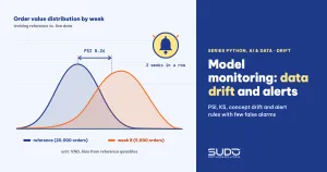
Data drift is what happens when the distribution of the inputs to a live model slowly moves away from the distribution of the data it was trained on. The model raises no error, the API still returns HTTP 200, latency looks great, yet prediction quality may be sliding week after week. This article builds a small monitoring system for a model that predicts whether a cash-on-delivery (COD) order will be refused by the customer: it measures data drift with PSI, KS, Wasserstein and chi-square, treats concept drift separately, designs alert rules with few false alarms, and then exports the measurements to Prometheus.
It follows MLOps with MLflow: experiment tracking, the model registry and deployment (the model already has a registry and versions) and Serving AI models with FastAPI: batching, timeouts and monitoring (the service already has latency monitoring). Those two articles answer "is the model running?"; this one answers the harder question: "is the model still right?" Every number is real output on an Apple M4, 16 GB, Python 3.12 (package versions are in requirements.txt); the source code is in code/s7-51. The data is self-generated simulation, not real customer data.
Why a model breaks and nobody notices
At training time we have labels immediately: the order history already says which orders were refused. In production, labels arrive late. A COD order's outcome is known only a few days after delivery, and a loan's repayment outcome only after many months. During that delay we have only the inputs and the predictions. That is why monitoring has two layers:
- The early layer, no labels needed: track the distribution of each feature, the distribution of prediction scores and the rate of missing values. This is where data drift is detected.
- The late layer, labels needed: once labels arrive, recompute AUC, log loss and calibration. This is where concept drift shows up.
The early layer is cheap but only an indirect signal: a changed distribution does not necessarily mean a worse model. The late layer is accurate but slow. A serious monitoring system uses both and knows which question each layer answers.
Data drift, covariate shift and concept drift compared
Terminology in the literature is quite muddled, so this article separates the cases by probability distribution. Let X be the features and y the label:
| Type | What changes | COD order example | Detected by |
|---|---|---|---|
| Data drift / covariate shift | P(X) changes, P(y|X) stays the same | Order values rise after a promotion season, the share of each city shifts | Comparing input distributions, no labels needed |
| Concept drift | P(y|X) changes | A new promotion brings many "fake" orders that get refused even though the old features did not change | Quality metrics once labels are available |
| Label shift | P(y) changes | The return rate rises across the whole system | The prediction score distribution, then labels |
The academic survey of concept drift (Lu et al., Learning under Concept Drift: A Review) splits the problem into detecting, understanding and adapting to drift. This article mostly covers the detection of data drift.
Simulated data and the reference model
The task: predict whether a COD order is refused. The features are the order value (VND), the number of items, the city (HCM, HN, DN, Other), the number of previous refusals and a promotion flag. The make_batch function generates the data and lets us switch on each kind of data drift in a controlled way: value_shift multiplies the order value, city_probs changes the share of each city, and concept changes the relationship between the features and the label.
The reference set is 20,000 orders from training time, with a refusal rate of 11.4%. One important rule: the reference set must be stored together with the model version (for example as an MLflow artifact, as in the previous article), because "data drift compared to what?" needs a fixed answer. If you use a sliding window as the reference, slow data drift "drifts along" with it and is never detected.
Four ways to measure the distance between two distributions
No single metric is best for every case; the four metrics below are in drift_metrics.py.
PSI: the population stability index
PSI (Population Stability Index) splits the reference data into bins (here 10 quantile bins), then sums (q - p) * ln(q / p) over the bins, where p and q are the proportions in the reference and in the new data. PSI has long been popular in credit scoring. The common thresholds are: below 0.1 is stable, 0.1 to 0.25 is worth a look, above 0.25 is a large shift. This is an industry convention, not a statistical standard, so calibrate it to your own data. You need to clip the minimum proportion (eps) so an empty bin does not make ln blow up.
def psi_numeric(ref, cur, bins=10, eps=1e-4):
    edges = np.quantile(ref, np.linspace(0, 1, bins + 1))
    edges[0], edges[-1] = -np.inf, np.inf
    p = np.histogram(ref, edges)[0] / len(ref)
    q = np.histogram(cur, edges)[0] / len(cur)
    p, q = np.clip(p, eps, None), np.clip(q, eps, None)
    return float(np.sum((q - p) * np.log(q / p)))
The bins must be computed from the reference, and the two outermost bins extend to infinity.
KS: the two-sample Kolmogorov–Smirnov test
The KS statistic is the largest distance between two empirical cumulative distribution functions. According to the SciPy documentation, the null hypothesis of ks_2samp is that both samples come from the same distribution. With method='auto', if both sample sizes are below 10,000 it tries to compute an exact p-value; otherwise (a single sample of 10,000 or more is enough) it uses an asymptotic approximation. The sample pairs in this article (for example 20,000 and 5,000) all use the asymptotic approximation. KS gives both a distance (0 to 1) and a p-value, but the p-value is exactly the trap covered in a later section.
Wasserstein: "how far must it move"
The Wasserstein-1 distance is the minimum effort needed to turn one distribution into the other, expressed in the units of the feature. Dividing it by the standard deviation of the reference (the W/σ column in this article) gives a unitless number: "how many standard deviations the data has shifted". When measuring data drift, this metric does not fall into the "always significant at large n" trap of the p-value, so it is a good fit for thresholds; at small sample sizes it is still noisy (see n=1,000 in experiment B).
Chi-square for categorical variables
For the city, we use PSI on the categories (same formula) and an independent chi-square test on a 2-row table (reference, current) by the number of categories.
Real run: eight weeks of data, two waves of data drift
Each week is a batch of 5,000 orders compared against the 20,000-order reference. From week 4 the order value rises 15%; from week 6 it rises 35% and the share of the city "Other" grows from 25% to 40%. Real output of demo_drift.py:
reference: 20000 orders, refusal rate = 0.114
week  PSI_value  KS     p(KS)    W/σ  PSI_city    chi2 p
   1    0.003  0.012  6.18e-01  0.018     0.001  5.27e-01
   2    0.002  0.017  1.75e-01  0.030     0.001  4.88e-01
   3    0.003  0.011  7.14e-01  0.022     0.000  9.21e-01
   4    0.054  0.093  7.50e-31  0.214     0.001  2.06e-01
   5    0.065  0.112  9.05e-44  0.247     0.000  8.95e-01
   6    0.230  0.205 2.25e-147  0.508     0.111  3.04e-101
   7    0.235  0.203 5.42e-145  0.508     0.096  3.07e-87
   8    0.239  0.207 3.84e-150  0.525     0.113  9.69e-104
How to read it: in the first three weeks every metric is close to 0. In weeks 4 and 5 the price rises 15%: the KS p-value is already as small as 1e-31, but PSI is only 0.054 and 0.065, still below the 0.1 threshold. This is the point to remember: a tiny p-value does not mean large data drift; it only means we are sure there is a difference. From week 6, the price PSI jumps to 0.23 and the city PSI to 0.11, while the city chi-square from week 4 to 5 still detects nothing (large p) because the city had not changed yet, exactly as the data was generated.
The sample-size trap: a p-value is not a measure of magnitude
With enough data, every difference, however small, is statistically significant. Conversely, with too small a sample, real data drift does not reach p < 0.05 either. Two experiments in demo_false_alarm.py illustrate both sides:
A) 200 comparisons of two batches from the SAME distribution (n=5,000): drift rate at p<0.05
   false alarms: 12/200
B) Very small shift (price +1%), growing sample size
        n      p(KS)     PSI    W/σ
     1000   5.53e-02  0.0071  0.052
     5000   8.57e-01  0.0006  0.011
    50000   5.79e-02  0.0003  0.016
   200000   2.44e-07  0.0004  0.020
Experiment A: two batches from the same distribution, yet 12 out of 200 times (6%) still get flagged as data drift, consistent with the 5% significance level we chose. Testing 30 features every day at a 0.05 threshold gives, on average, one to two false alarms per day; you must correct for it (Bonferroni) or use a distance threshold instead of a p-value. Experiment B: a price shift of only 1% pushes the p-value down to 2.4e-07 at n = 200,000, while PSI stays at 0.0004, completely harmless. The fluctuating rows at small n are sampling noise.
That is why real monitoring tools pick the method by sample size. According to the Evidently documentation, for a reference set of 1,000 rows or fewer they use tests (KS for numeric features, chi-square for categorical ones, threshold p = 0.05); for larger sets they switch to distances (Wasserstein for numeric features, Jensen–Shannon for categorical ones, threshold 0.1). The rule to take away: with a large sample, set the threshold on the magnitude of the data drift, not on the p-value.
Concept drift: when the inputs do not change but the model is still wrong
Data drift is not always harmful, and a model can break without the inputs shifting. To see this clearly, demo_concept.py trains a HistGradientBoostingClassifier on the reference and then scores it on five scenarios once labels are available:
holdout: AUC=0.659
scenario                    PSI_value  PSI_city    AUC  logloss  mean predicted rate  actual rate
stable                        0.003     0.002  0.662    0.333             0.114      0.111
covariate: price +35%         0.259     0.001  0.667    0.353             0.124      0.123
covariate: city mix changed   0.003     0.115  0.668    0.349             0.120      0.121
concept: promotion (0.8)      0.004     0.001  0.581    0.407             0.112      0.140
concept: promotion (1.5)      0.003     0.001  0.527    0.536             0.116      0.195
This is the most important table in the article. The two covariate drift rows have PSI of 0.259 and 0.115, above the warning threshold, but AUC does not drop (0.667 and 0.668, on par with the 0.662 of the stable scenario) and the mean predicted rate tracks the actual rate closely: the model is still right because the relationship P(y|X) did not change and it had learned to generalize over price and city. The two concept drift rows are the opposite: the feature PSI is only 0.004 and 0.001, so the input data drift alarm stays completely silent, yet AUC falls from 0.662 to 0.581 and then 0.527 (close to guessing), and the actual refusal rate is 0.195 while the model still predicts 0.116.
The design consequence: data drift is a sufficient reason to investigate, not a sufficient reason to retrain; and not seeing data drift does not prove the model is healthy. To catch concept drift, you need late labels flowing back and quality recomputed over windows (weekly, monthly), together with a comparison of the mean predicted rate against the actual rate. The base AUC is low (0.66) because the simulated data is noisy; the differences between scenarios are what you should read.
With high-dimensional features (embeddings, images, text), comparing dimension by dimension is meaningless. The study Failing Loudly (Rabanser, Günnemann, Lipton, NeurIPS 2019) reports that a two-sample test after dimensionality reduction with a trained classifier is the strongest method among the kinds of shift they tried; this article does not run that method.
Designing alerts: few false alarms, clear actions
The worst alerting system is one that gets muted after two weeks because it pages too much. Four principles apply to data drift:
- Two levels:
warning(PSI from 0.1) goes to the dashboard; exceeding the warning threshold for two consecutive periods, or reachingcritical(from 0.25), pages a person. Each level is tied to a specific action. - Require persistence: page someone only after the threshold is exceeded for at least two consecutive periods; a single odd batch (a holiday, a flash sale) should not wake anyone up.
- Alert on important features: rank features by their contribution to the model (see Explaining models with SHAP: understanding why a model decides); for a feature with almost no influence, its data drift is for reference only.
- Have a cross-check: pair every data drift alert with a quality metric once labels are available (previous section), because input data drift alone often over-reports.
alerts.py simulates this rule on the same eight weeks and exports the measurements through prometheus_client. The Gauge carries the labels model and feature so one dashboard can serve many models. Real output:
week feature         PSI level   consecutive  action
   6 order_value   0.230 warning           1
   6 city          0.111 warning           1
   7 order_value   0.235 warning           2  PAGE: check the pipeline, consider retraining
   8 order_value   0.239 warning           3  PAGE: check the pipeline, consider retraining
   8 city          0.113 warning           1
--- /metrics (week 8) ---
# HELP model_feature_psi PSI against the reference set
# TYPE model_feature_psi gauge
model_feature_psi{feature="order_value",model="cod_refuse_v3"} 0.23908754601725812
model_feature_psi{feature="city",model="cod_refuse_v3"} 0.11279629806330294
Weeks 4 and 5 (PSI 0.054 and 0.065) raise no alert even though KS already has a tiny p-value: that is deliberate. In week 6 the order value has PSI 0.230, still below the critical threshold of 0.25, so it is only a warning; week 7 is the second consecutive period, so only then does it "PAGE" (in the eight simulated weeks no period reached the critical level of 0.25, so the critical branch for data drift does not appear in the output). The city has PSI 0.111, 0.096 and then 0.113: it hovers around the threshold so the streak resets, which is why real systems add a buffer zone (hysteresis) or a moving average.
Exporting to Prometheus and Grafana
If your infrastructure already has Prometheus, as in Kubernetes monitoring with kube-prometheus and Grafana, you need no new tool. A scheduled job computes PSI every day and updates the Gauge; a long-running process opens a port with start_http_server as described in the prometheus_client documentation. For short-lived jobs, use the Pushgateway. The "two consecutive periods" rule can be moved into Prometheus with the for clause in alerting rules: the alert stays pending until the condition holds for the whole for duration, and keep_firing_for keeps the alert firing a little longer to avoid flapping.
groups:
- name: model-drift
  rules:
  - alert: FeatureDriftSustained
    expr: model_feature_psi{model="cod_refuse_v3"} > 0.1
    for: 2d
    keep_firing_for: 1d
    labels:
      severity: page
    annotations:
      summary: "PSI {{ $labels.feature }} above 0.1 for 2 days in a row"
This YAML configuration was not run in this article (the test machine has no Prometheus); validate it with promtool check rules before loading it. For a data drift dashboard and alerts, see Grafana Alerting for pods: RAM dashboards, alerts and the ingress-nginx ServiceMonitor.
What to do when data drift happens
In order from cheapest to most expensive: (1) rule out data errors, because most data drift is really a broken pipeline (a unit change from VND to thousands of VND, a new column that is all null, a city code that changed format); (2) check whether the data drift is harmful, using quality metrics once labels are available or SHAP to see how important that feature is; (3) recalibrate the probabilities or change the decision threshold; (4) retrain on recent data, register the new version in the registry (see the MLflow article) and compare it with the old one using the metrics in Model evaluation for classifiers: precision, recall, ROC and imbalanced data before switching over.
Do not retrain automatically just because a data drift alert fired. The table above has two scenarios where the inputs shifted yet the model stays right; retraining there only adds risk. Recent data may also contain the very effect you want to avoid, such as "fake" orders caused by a promotion, so review the labels first.
Common mistakes
- Taking bins from the new data instead of the reference: PSI is always low because the bins adapt themselves. Forgetting to extend the two edge bins to infinity also hides the most dangerous kind of data drift, values outside the training range.
- Using the p-value as a measure of magnitude at large sample sizes, or testing many features without correction: false alarms every day.
- Using a sliding window as the reference: slow data drift is never detected. Monitoring only the inputs also lets concept drift slip through.
- Logging predictions together with personal data: monitoring only needs anonymized features or aggregate statistics.
Checklist
- Store the reference set with every model version; track the distribution of the important features, the prediction scores and the missing rate.
- Use tests for small samples and distances (PSI, Wasserstein) for large ones; alert on two levels, on consecutive threshold breaches, with a named owner.
- When labels arrive, compute quality over windows to catch harmful data drift and concept drift; do not retrain automatically.
Setup: python3.12 -m venv .venv && .venv/bin/pip install -r requirements.txt, then run demo_drift.py, demo_false_alarm.py, demo_concept.py and alerts.py in code/s7-51; the *_output.txt files are the pasted output. Each script runs in under a minute and uses under 200 MB of RAM.
Next article
Responsible AI: personal data, bias and Vietnam's Decree 13 on data protection. Monitoring tells us whether the model is still right; the next article asks whether the data used for training and monitoring may be used at all, and whether the model treats groups of customers fairly.