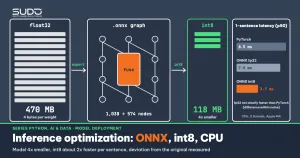
ONNX (Open Neural Network Exchange) is an open format for storing a machine learning model as a computation graph plus weights, separate from the framework that trained it. An ONNX model runs on ONNX Runtime, an inference engine written in C++ with its own providers for CPU, GPU and a range of other hardware. This article takes a multilingual embedding model that is already used for Vietnamese search, exports it to ONNX, optimizes the graph, quantizes it to int8, and measures what you gain and what you lose on a CPU.
It follows Serving AI models with FastAPI: batching, timeouts and monitoring: once the service has batching and monitoring, the next question is how to make each inference cheaper. The model is paraphrase-multilingual-MiniLM-L12-v2, the same one used in Embeddings and semantic search. Every number in the article is real output on an Apple M4 with 16 GB, Python 3.12, torch==2.8.0 and onnxruntime==1.23.2; the source code is in code/s7-48. The machine has no NVIDIA GPU, so the article covers CPU only; the GPU path (TensorRT, CUDA provider) was not run.
Why optimize inference on a CPU
A lot of real enterprise workloads are small models running steadily: embeddings for search, ticket classification, risk scoring, rerankers. These models fit in the RAM of an ordinary server, and the main costs are latency and the number of CPUs you rent. For a model of this size, depending on the hardware and load, a CPU may be enough and you may not need a GPU at all. In this article the quantized model is four times smaller and about twice as fast for a single sentence on an Apple M4; it was not measured on an x86 VPS, so do not assume those numbers carry over to your machine.
There are three different levers: change the runtime (PyTorch to ONNX Runtime, with graph optimization), reduce numeric precision (float32 to int8) and tune how it runs (thread count, padding length). The article measures each lever separately to see which one actually helps.
What ONNX is and where it sits in the deployment chain
An ONNX file is a protobuf containing a list of inputs/outputs with types and shapes, a list of nodes (each node is an operator such as MatMul, Add or Softmax), a list of initializers (the weights) and the opsets that state which version of the operator specification is used. Because the graph is frozen, the runtime can analyze all of it, fuse nodes and pick the best kernels for the CPU, something the Python loop of eager PyTorch cannot do.
The trade-off with ONNX: you add a conversion step that is easy to break (unusual operators, dynamic control flow, a tokenizer that still lives outside the graph), and you must verify that the results do not change. The rest of the article is that verification process.
Step 1: export the model to ONNX
We wrap the model in an Embedder that includes mean pooling and L2 normalization, so the ONNX file takes input_ids and attention_mask and returns the 384-dimensional vector directly. Moving the post-processing into the graph means there is no separate NumPy code to keep in sync with training.
class Embedder(torch.nn.Module):
    def __init__(self, base):
        super().__init__(); self.base = base
    def forward(self, input_ids, attention_mask):
        h = self.base(input_ids=input_ids, attention_mask=attention_mask).last_hidden_state
        m = attention_mask.unsqueeze(-1).to(h.dtype)
        v = (h * m).sum(1) / m.sum(1).clamp(min=1e-9)
        return torch.nn.functional.normalize(v, dim=-1)

torch.onnx.export(
    model, (enc["input_ids"], enc["attention_mask"]), "embedder_fp32.onnx",
    input_names=["input_ids", "attention_mask"], output_names=["embedding"],
    dynamic_axes={"input_ids": {0: "batch", 1: "seq"},
                  "attention_mask": {0: "batch", 1: "seq"},
                  "embedding": {0: "batch"}},
    opset_version=17, dynamo=False)
onnx.checker.check_model(onnx.load("embedder_fp32.onnx"))
Two details matter. First, dynamic axes: if you do not declare dynamic_axes, the ONNX file hard-codes the batch size and length of the sample input, and any sentence of a different length will fail or return wrong results. Second, choosing the exporter: the article uses PyTorch 2.8, where the TorchScript-based exporter is the default. According to the PyTorch documentation, from version 2.9 the dynamo parameter defaults to True (the torch.export-based exporter) and dynamic_shapes is meant for that path, while dynamic_axes is used with dynamo=False. That is why I set dynamo=False explicitly here; if you upgrade PyTorch to 2.9 or later without setting it, the export path will differ, so rerun the verification step below. Real output:
opset: [('ai.onnx', 17)] ir_version: 8
nodes: 1038 | initializers: 197
top op: [('Constant', 308), ('Add', 122), ('MatMul', 96), ('Unsqueeze', 70), ('Mul', 51), ('Concat', 50), ('Reshape', 50), ('Transpose', 48)]
size: 470.2 MB
The notable number is in the weights. The script step6_dynamic_check.py counted 117,653,760 parameters, of which the vocabulary embedding table alone (word_embeddings, 250,037 tokens × 384 dimensions) accounts for 96,014,208, or 81.6%. The rest, where the MatMul operations of the 12 transformer layers live, is only about 21.6 million. The vocabulary lookup table costs almost no computation but takes most of the file size, so whether quantization touches it (see step 3) decides the file size.
Step 2: graph optimization in ONNX Runtime
According to the ONNX Runtime documentation, there are three groups of graph optimizations, and each level includes the previous ones: basic (constant folding, removing redundant nodes), extended (fusing more complex nodes such as MatMul+Add, LayerNorm and Attention, for CPU/CUDA/ROCm only) and layout (changing the data layout, CPU only). ORT_ENABLE_ALL turns on all three and is the default. We write the optimized graph to a file at each level and count nodes:
so = ort.SessionOptions()
so.graph_optimization_level = ort.GraphOptimizationLevel.ORT_ENABLE_EXTENDED
so.optimized_model_filepath = "embedder_fp32_extended.onnx"
ort.InferenceSession("embedder_fp32.onnx", so, providers=["CPUExecutionProvider"])
onnxruntime 1.23.2
disable node= 729 470.2 MB
basic node= 634 470.2 MB
extended node= 574 470.2 MB
all node= 574 470.2 MBThe node count drops from 1,038 (the exported file) to 574, almost half, but the file size does not change: graph optimization only rearranges the computation and never touches the weights. Even at the disable level the count is already 729, not 1,038. The extended and all levels end at the same 574 nodes because the model contains no operators that depend on the NCHWc layout (a layout type meant for convolutions).
When you write an optimized model to disk, ONNX Runtime prints this real warning for levels above extended:
Serializing optimized model with Graph Optimization level greater than ORT_ENABLE_EXTENDED and the NchwcTransformer enabled. The generated model may contain hardware specific optimizations, and should only be used in the same environment the model was optimized in.The practical consequence: do not save a file optimized at the all level and move it to another machine. The safe approach is to ship the original ONNX file and let each machine optimize it when it loads the session (a few hundred milliseconds, see the load-time table below).
Step 3: dynamic int8 quantization
Quantization replaces float32 weights (4 bytes) with 8-bit integers plus a scale factor. ONNX Runtime has two kinds. Dynamic quantization quantizes only the weights at conversion time and computes the activation scale during inference. Static quantization uses calibration data to fix that scale in advance. According to the ONNX Runtime quantization documentation, use the dynamic kind for transformers and RNNs and the static kind for CNNs. The dynamic kind needs no calibration data, which makes it the simplest starting point:
from onnxruntime.quantization import quantize_dynamic, QuantType
quantize_dynamic("embedder_fp32.onnx", "embedder_int8.onnx", weight_type=QuantType.QInt8)
int8: node=1305 118.1 MB
quantized ops: [('DynamicQuantizeLinear', 48), ('MatMulInteger', 72)]The file is exactly 4 times smaller: 470.2 MB down to 118.1 MB. Inspecting it with onnx shows that even the vocabulary embedding table became 8-bit integers (real output of step6_dynamic_check.py: the largest initializer is base.embeddings.word_embeddings.weight_quantized, type UINT8, shape [250037, 384]), so all the large weights shrink. The graph has more nodes (1,305 versus 1,038) because every MatMul gets an extra activation-quantization node (DynamicQuantizeLinear) and is converted to MatMulInteger. The tool warns that you should run a preprocessing step first; the article skips it, so accuracy may not be at its best.
Step 4: verify that ONNX gives the same results as PyTorch
Measuring speed before measuring correctness is the fastest way to optimize a model into a broken one. The script step3_parity.py compares three variants on the same 12 documents and 8 Vietnamese queries (with hand-labeled correct answers). It measures the largest absolute vector deviation, the smallest cosine between the original vector and the variant vector, then top-1 and top-3 retrieval:
model      max|Δ| doc     cos min doc    top-1    top-3
torch      0.00e+00       1.000000       0.75     1.00
onnx fp32  2.51e-07       1.000000       0.75     1.00
onnx int8  3.53e-02       0.977287       0.75     1.00

fp32: single sentence vs in a padded batch, max|Δ| = 0.00e+00
int8: single sentence vs in a padded batch, max|Δ| = 1.35e-02
torch      cosine score of correct pairs: 0.564 0.244 0.853 0.745 0.605 0.630 0.359 0.806
onnx fp32  cosine score of correct pairs: 0.564 0.244 0.853 0.745 0.605 0.630 0.359 0.806
onnx int8  cosine score of correct pairs: 0.549 0.247 0.847 0.729 0.577 0.624 0.343 0.798
Reading the results:
- ONNX fp32 is almost identical to PyTorch: the largest deviation is 2.5×10⁻⁷, at the level of float32 rounding error.
- int8 deviates more visibly: the largest per-dimension deviation is 0.035, the most-shifted vector still has a cosine of 0.977 against the original, and the cosine score of the correct pair drops by roughly 0.006 to 0.028 on 7 of the 8 queries (one query rises by 0.003).
- The retrieval ranking does not change: all three give top-1 = 0.75 and top-3 = 1.00. Do not read too much into it, though: 8 queries is far too few to conclude anything about quality. A real test set needs a few hundred queries taken from your own system's logs, as in RAG evaluation.
- int8 results depend on the batch: the same sentence produces different vectors (deviating by up to 0.0135) when it is alone versus inside a padded batch of 12 sentences, while fp32 deviates by exactly 0. This matches how dynamic quantization works: the activation scale is computed over the whole tensor at inference time, so the neighboring sentences influence yours. I have not isolated this cause with a separate experiment, but the consequence is real: a system that stores precomputed vectors should use one fixed inference mode and should not mix vectors from two variants.
Step 5: measure CPU latency
Measuring latency has more traps than it seems. My machine is shared with many other processes, and the first time I ran this the load average was above 20 on 10 cores: absolute numbers were 3 to 7 times higher and the order between configurations changed too. So step4_bench.py runs each configuration interleaved in the same loop, with a warm-up, torch.set_num_threads(2) and intra_op_num_threads = 2 on both sides, then repeats the whole measurement block 5 times and reports the median together with the spread across rounds. I waited until the load average fell below 9 before the final run. Real output:
batch=1 (5 rounds x 40 iterations)
  PyTorch fp32           min   5.1  p50   8.5 (rounds:   5.4-  9.3)  p95  37.5 ms  | vs PyTorch: 1.00x (1.00-1.00)
  ORT fp32 (no opt)      min   6.1  p50   7.1 (rounds:   6.5- 10.5)  p95  12.4 ms  | vs PyTorch: 0.84x (0.82-1.23)
  ORT fp32 (ALL)         min   6.1  p50   7.5 (rounds:   7.4-  9.7)  p95  14.6 ms  | vs PyTorch: 0.90x (0.72-1.14)
  ORT int8 dynamic       min   2.4  p50   3.7 (rounds:   3.6-  4.3)  p95   8.1 ms  | vs PyTorch: 2.02x (1.49-2.37)
batch=12 (5 rounds x 15 iterations)
  PyTorch fp32           min  19.8  p50  21.1 (rounds:  18.1- 22.8)  p95  33.4 ms  | vs PyTorch: 1.00x (1.00-1.00)
  ORT fp32 (no opt)      min  59.6  p50  63.9 (rounds:  56.5- 70.9)  p95  78.7 ms  | vs PyTorch: 0.33x (0.32-0.33)
  ORT fp32 (ALL)         min  58.2  p50  61.5 (rounds:  54.5- 64.1)  p95  97.2 ms  | vs PyTorch: 0.34x (0.33-0.36)
  ORT int8 dynamic       min  21.0  p50  22.5 (rounds:  19.6- 24.1)  p95  33.5 ms  | vs PyTorch: 0.94x (0.91-1.00)
load average start/end: 8.8 19.1 21.1 -> 8.3 18.1 20.7
The "vs PyTorch" column is the p50 ratio (above 1 means faster than PyTorch); the numbers in parentheses are the spread across the 5 rounds. Observations from the measurements:
- For a single sentence, ONNX Runtime fp32 is not consistently faster than PyTorch: p50 of 7.5 ms versus 8.5 ms, a ratio of 0.90x with a spread of 0.72 to 1.14 that lies on both sides of 1. Someone rerunning on a less loaded machine even saw fp32 come out slower than PyTorch. The safe conclusion is that the two are even within the noise; int8 is the fastest variant, with a p50 of 3.7 ms, about 2 times faster (1.5 to 2.4 times across rounds).
- With a batch of 12 sentences, ONNX Runtime fp32 is about three times slower than PyTorch (61.5 ms versus 21.1 ms, ratio 0.34x). This repeated in every measurement and every round, even when the machine was busy. No lever is automatically right: on this machine, with a large batch, the ONNX Runtime fp32 path loses to PyTorch. I have not found the cause, so I only report the measurement; on an x86 server the result may be quite different.
- int8 at batch 12 is on par with PyTorch (22.5 versus 21.1 ms, ratio 0.94x, spread 0.91 to 1.00): the speed advantage is gone and only the size advantage remains. The clearest benefit of int8 is the one-sentence-per-call case.
- Graph optimization ALL versus off: no difference within the noise at batch 1 (7.5 versus 7.1 ms) and batch 12 (61.5 versus 63.9 ms).
For memory and startup time, step5_size_load.py measured three consecutive loads of each file:
embedder_fp32.onnx    470.2 MB  session load: 152 / 107 / 104 ms
embedder_int8.onnx    118.1 MB  session load: 80 / 69 / 61 ms
Load time fluctuates with the operating system's cache and machine load, so I only draw a conclusion about size: for a Kubernetes pod with many replicas on small nodes (see requests and limits), the 118 MB file saves far more RAM and image-pull bandwidth than the 470 MB file.
Using ONNX Runtime in a real service
A session (InferenceSession) is safe to share across threads, so create it once when the service starts and reuse it, not on every request. A minimal embed function to drop into the FastAPI endpoint from the previous article:
import onnxruntime as ort
from transformers import AutoTokenizer

tok = AutoTokenizer.from_pretrained(MODEL_ID)
so = ort.SessionOptions()
so.intra_op_num_threads = 2          # match the vCPUs allocated to the pod
sess = ort.InferenceSession("embedder_int8.onnx", so, providers=["CPUExecutionProvider"])

def embed(texts: list[str]):
    enc = tok(texts, padding=True, truncation=True, max_length=128, return_tensors="np")
    return sess.run(None, {"input_ids": enc["input_ids"],
                           "attention_mask": enc["attention_mask"]})[0]
According to the ONNX Runtime threading documentation, if you do not set intra_op_num_threads it defaults to the number of physical cores, and setting it explicitly turns off thread affinity to cores. In a container, set it explicitly to match the pod's CPU limit. Also truncate the input (truncation=True, max_length=128): padding length is a major speed parameter that many people forget, because attention cost grows with the square of the length.
When not to use ONNX or quantization
- When you have no quality test set yet. Without a set of queries with known answers you cannot tell what int8 breaks. Build the test set first, as in the LLM evaluation article.
- When the load is small. 4 ms versus 15 ms for one sentence does not decide the user experience if you only get a few requests per second.
- When the model has dynamic control flow or custom operators, the ONNX export may fail or produce a different graph. Text-generating LLMs use a KV cache and run token by token, which needs other tools (llama.cpp in the article on running a local LLM, or vLLM in the next article).
- When you need a GPU. The article measures CPU only. Running ONNX Runtime on a GPU (CUDA or TensorRT provider) needs NVIDIA hardware that the test machine does not have; that part needs a GPU and was not run in the article.
Common mistakes
- Forgetting dynamic axes: the model only works correctly with the batch size and length of the sample input. Test with other lengths (this article checks it with
step6_dynamic_check.py: a 4-token sentence and a 62-token sentence both return a 384-dimensional vector). - Changing the PyTorch version without rechecking: from 2.9 the default exporter changes and so does the way dynamic axes are declared (
dynamic_shapesinstead ofdynamic_axes); pin the version inrequirements.txtand rerun the verification step.
CPU inference optimization checklist
- Export ONNX together with any pre/post-processing that can go into the graph (pooling, normalization), declare dynamic axes, run
onnx.checker. - Compare with PyTorch by numeric deviation and, more importantly, by your business metric on a separate test set.
- Try dynamic int8 quantization for transformers; look at size, latency and quality together.
- Set
intra_op_num_threadsto the CPU limit, create the session once, truncate the input length. - Measure p50 and p95 on real batches and real hardware: x86 and ARM give different results.
Setup: python3.12 -m venv .venv && .venv/bin/pip install -r requirements.txt, then run export_onnx.py, optimize_quantize.py, step3_parity.py, step4_bench.py and step5_size_load.py in code/s7-48; the *_output.txt files are the pasted output. Primary documentation: ONNX Runtime quantization, graph optimizations and the PyTorch ONNX exporter.
Next article
Self-hosting LLMs with vLLM: continuous batching and the KV cache. A small embedding model runs well on a CPU, but a text-generating model has a very different problem: KV cache memory and request scheduling decide throughput.