Polars is a DataFrame library written in Rust with a Python API, built around one idea: you describe the whole query first, the library optimizes the plan, and only then does it read any data. On an orders table with a few million rows, this approach makes a very clear difference compared with the usual pandas habit of loading the whole file into memory and processing it step by step. This article runs the same revenue report on 5 million simulated order rows with pandas 3.0 and Polars 1.42, measures run time and peak RAM, reads the query plan (explain), and then says plainly when you should and should not switch to Polars.
This article builds on the two earlier articles in the series about tabular data processing: Cleaning data with pandas and NumPy vectorization and broadcasting. Environment: Apple M4, 16 GB RAM, Python 3.12, polars==1.42.1, pandas==3.0.3, pyarrow==25.0.0, numpy==2.5.1; the source code is in code/s7-53. The data is simulated and self-generated, not real customer data. The machine was running other tasks at the time, so every timing is the median of 5 runs and is only meaningful as a relative comparison.
The problem: a report that runs on a laptop runs out of RAM when the data grows tenfold
This is a familiar scenario in a retail business: the daily order export is accumulated into a CSV of a few hundred MB, and someone writes a pandas notebook to produce a revenue report by city and sales channel. The notebook works well with one quarter of data. When the data grows to a full year, it gets much slower and RAM starts to be a problem. The cause is usually not that pandas is "bad", but the execution model: every line of code runs immediately (eager), reads all columns, and creates extra intermediate copies.
Polars addresses this with three things you can verify: lazy execution with a query optimizer, an execution engine that runs expressions in parallel, and (in recent releases) batch-wise execution (streaming). According to the Polars documentation on data types, Polars uses the Arrow columnar format for memory, but the documentation also says the performance comes mainly from the query engine, plan optimization, and parallel expression execution, not only from the memory layout.
The simulated data and the query used for comparison
The gen_data.py script generates an orders table with 9 columns: order_id, customer_id, order_date, city, channel, sku, qty, unit_price, status. With 5 million rows, the CSV file is 280 MB and the compressed Parquet file is only 49.5 MB. The measured query is a typical report: take paid orders since April 1, 2026, compute revenue, group by city and channel, and keep the 5 groups with the highest revenue.
import polars as pl
from datetime import date

def query(lf):
    return (lf.filter((pl.col("status") == "paid") & (pl.col("order_date") >= date(2026, 4, 1)))
              .with_columns(revenue=pl.col("qty") * pl.col("unit_price"))
              .group_by("city", "channel")
              .agg(orders=pl.len(), revenue=pl.col("revenue").sum(), avg_qty=pl.col("qty").mean())
              .sort("revenue", descending=True).head(5))

out = query(pl.scan_csv("orders.csv", try_parse_dates=True)).collect(engine="in-memory")
The pandas version does the same job in the familiar way: read_csv, filtering with a boolean mask, assign, groupby().agg(). In every run mode, the first row of the result is identical (HCM, web, 275,043 orders, revenue 196,076,218,000 VND), so the comparison is fair in terms of results.
The lazy API: scan, query plan, and collect
The core difference is read_csv versus scan_csv. pl.read_csv reads immediately and returns a DataFrame. pl.scan_csv only returns a LazyFrame, a "promise of computation"; no row of data is read until you call .collect(). According to the Execution page of the Polars documentation, each line of code is added to an internal query graph, and that graph is optimized before it runs.
We can look at the plan before and after optimization with explain. The real output of demo_explain.py:
=== explain(optimized=False) ===
SLICE[offset: 0, len: 3]
  SORT BY [descending: [true]] [col("revenue")]
    AGGREGATE[maintain_order: false]
      [len().alias("orders"), col("revenue").sum()] BY [col("city"), col("channel")]
      FROM
       WITH_COLUMNS:
       [[(col("qty")) * (col("unit_price"))].alias("revenue")]
        FILTER [(col("order_date")) >= (2026-04-01)]
        FROM
          FILTER [(col("status")) == ("paid")]
          FROM
            Csv SCAN [orders.csv]
            PROJECT */9 COLUMNS
            ESTIMATED ROWS: 5609054
=== explain() (optimized) ===
SORT BY [slice: (0, 3, dynamic_pred: cbf69941-1418-49a9-bc0b-32fe3ee57421), descending: [true]] [col("revenue")]
  FILTER col("revenue").dynamic_predicate()
  FROM
    AGGREGATE[maintain_order: false]
      [len().alias("orders"), col("revenue").sum()] BY [col("city"), col("channel")]
      FROM
      simple π 3/3 ["city", "channel", "revenue"]
         WITH_COLUMNS:
         [[(col("qty")) * (col("unit_price"))].alias("revenue")]
          simple π 4/4 ["city", "channel", "qty", ... 1 other column]
            Csv SCAN [orders.csv]
            PROJECT 6/9 COLUMNS
            SELECTION: [([(col("order_date")) >= (2026-04-01)]) & ([(col("status")) == ("paid")])]
            ESTIMATED ROWS: 5609054
Three changes stand out in the optimized plan. First, PROJECT 6/9 COLUMNS: only 6 of the 9 columns are read from the file (projection pushdown), and the order_id, customer_id, and sku columns are never loaded. Second, SELECTION sits right at the scan step: the two filters are merged into one and applied while reading (predicate pushdown), so rows that fail the condition are dropped early. Third, SORT BY [slice: ...] with dynamic_predicate: because only the top N rows are needed, Polars folds head into the sort step instead of sorting everything and then cutting. The full list of optimizations (predicate, projection, and slice pushdown, duplicate subquery elimination, expression simplification, join ordering, type coercion, cardinality estimation) is on the Optimizations page.
One less-mentioned benefit: the schema is inferred without reading any data. lf.collect_schema() immediately returns Schema({'city': String, 'channel': String, 'orders': UInt32, 'revenue': Int64}). A wrong column name or a type mismatch is caught before you spend time reading a large file.
Choosing an engine: in-memory versus streaming
According to the LazyFrame.collect documentation, the engine parameter accepts "auto", "in-memory", "streaming", or "gpu". The "auto" mode uses the engine set through Config.set_engine_affinity or the POLARS_ENGINE_AFFINITY environment variable, and with Polars 1.42 (the version used in this article) it falls back to "in-memory" if nothing is set; the docstring of this version says streaming "will soon become the default".
The stable documentation on the website always follows the latest Polars release, so it may describe a different default from the version you installed; check the docstring of the version you use (help(pl.LazyFrame.collect)). Streaming processes the query in batches instead of "in one block" like the in-memory engine, which reduces memory pressure; if the chosen engine cannot run a query, Polars falls back to in-memory automatically. The documentation marks GPU mode as unstable and it needs an Nvidia card plus cudf-polars; the machine in this article has no GPU, so that part needs a GPU and was not run in this article.
In this article I pass engine explicitly so the result does not depend on environment configuration. For data larger than RAM, the Execution documentation recommends engine="streaming", while stating clearly that Polars "may" process in batches and does not promise that every query can run this way; so try it on your real query instead of assuming.
Measured results: 5 million rows, one 16 GB machine
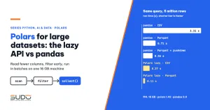
Each run mode is a separate Python process (bench.py <mode>) so that peak RAM (ru_maxrss) is not mixed up. The table below shows the median time of 5 runs and the peak RAM; the time includes both reading the file and computing.
| Run mode | Source | Time (s) | Peak RAM (MB) |
|---|---|---|---|
| pandas, read everything | CSV 280 MB | 3.31 | 1,397 |
| pandas, read everything | Parquet 49.5 MB | 0.71 | 1,315 |
pandas, read_parquet(columns=, filters=) | Parquet | 0.54 | 665 |
Polars read_csv then compute, optimizations off | CSV | 0.41 | 880 |
Polars lazy, engine="in-memory" | CSV | 0.37 | 628 |
Polars lazy, engine="streaming" | CSV | 0.32 | 550 |
Polars lazy, engine="in-memory" | Parquet | 0.11 | 281 |
Polars lazy, engine="streaming" | Parquet | 0.09 | 205 |
About measurement noise: the test machine is a shared machine, with a load average often above 20 on 10 cores. In an earlier measurement, the first pandas run reading Parquet took about 7.8 seconds, and when the machine was even busier, one pandas run took 38 seconds. I checked the suspicion that the cause was converting the order_date column from object to datetime64: the to_datetime step took only 0.56 seconds, so that was not the cause; it was most likely CPU and memory contention, and pandas, which uses more RAM, was affected more heavily. The table above was re-measured over 5 consecutive runs at a load average of about 8.7; bench_output.txt keeps every run. Treat the numbers as orders of magnitude, not absolute values.
How to read the results, carefully, so as not to overreach:
- For the same query, the difference in time is large: with CSV, pandas takes 3.31 seconds and Polars lazy about 0.37 seconds, roughly 9 times faster. Most of the gap comes from multi-threaded CSV reading and parsing and from parallel group-by.
- Lazy is not always faster than eager in time: the "optimizations off" row (0.41 seconds) and the lazy in-memory row (0.37 seconds) differ within the noise margin of a machine running other tasks. The clear benefit of lazy is in peak RAM: 628 MB versus 880 MB, because the 3 unused columns are not read.
- File format matters as much as the engine: switching from CSV to Parquet cut Polars peak RAM from 628 to 281 MB and cut the time by about 3 times, because Parquet is a columnar format, lets you read individual columns, and can skip whole row groups based on statistics.
- pandas can also push columns and filters down to the read step: when you call
read_parquetwithcolumnsandfilters(through PyArrow), pandas drops from 1,315 MB to 665 MB and from 0.71 to 0.54 seconds. The gap with Polars narrows but remains: 0.54 seconds versus 0.11 seconds and 665 MB versus 281 MB. - Streaming matters more when the data is large: with 5 million rows, streaming saves only about 12 to 27% more RAM (628 down to 550 MB with CSV, 281 down to 205 MB with Parquet) compared with in-memory. The real advantage is being able to run queries that do not fit in memory, which cannot be demonstrated on a shared machine.
When the thread count is limited with the environment variable POLARS_MAX_THREADS=2 (simulating a small container), the Polars lazy query on CSV takes 0.55 seconds and uses 515 MB; on Parquet it takes 0.13 seconds and uses 237 MB, still faster than pandas at the full core count (this is a single run, not a median; the last two lines of bench_output.txt). Keep this in mind when running in a container with a CPU limit.
Expressions, windows, and joins in one lazy graph
The real strength of Polars is expressions (pl.col(...)) that compose and run in parallel. The example below does three things in one graph: joins a regions table, ranks SKUs by revenue within each region using the window function .over("region"), and aggregates revenue by month with group_by_dynamic. The two results share the read and filter branch, so call pl.collect_all so that the shared branch is computed only once (exactly the recommendation in the Execution documentation for branching queries).
orders = pl.scan_parquet("orders_sink.parquet")
regions = pl.LazyFrame({"city": ["HCM", "HN", "DN", "CT", "HP", "Khac"],
                        "region": ["South", "North", "Central", "South", "North", "Other"]})
paid = (orders.filter(pl.col("status") == "paid")
        .with_columns(revenue=pl.col("qty") * pl.col("unit_price"))
        .join(regions, on="city", how="left"))

top_sku = (paid.group_by("region", "sku").agg(revenue=pl.col("revenue").sum())
           .with_columns(rank=pl.col("revenue").rank("dense", descending=True).over("region"))
           .filter(pl.col("rank") <= 2).sort("region", "rank"))
monthly = (paid.sort("order_date").group_by_dynamic("order_date", every="1mo", group_by="region")
           .agg(orders=pl.len(), revenue=pl.col("revenue").sum())
           .filter(pl.col("region") == "South").sort("order_date"))
a, b = pl.collect_all([top_sku, monthly])
The orders_sink.parquet file is produced from the CSV with pl.scan_csv(...).sink_parquet(...), a conversion that runs in batches and does not load the whole CSV file into a single DataFrame. The real output of demo_pipeline.py (shortened):
sink_parquet: 0.69 s, peak RAM 545 MB
collect_all: 0.37 s
┌────────┬─────────┬───────────┬──────┐
│ region ┆ sku     ┆ revenue   ┆ rank │
╞════════╪═════════╪═══════════╪══════╡
│ North  ┆ SKU1408 ┆ 530026000 ┆ 1    │
│ North  ┆ SKU1582 ┆ 519179000 ┆ 2    │
│ South  ┆ SKU1295 ┆ 680433000 ┆ 1    │
│ South  ┆ SKU0619 ┆ 677310000 ┆ 2    │
└────────┴─────────┴───────────┴──────┘
The peak RAM of 545 MB for sink_parquet shows that "streaming" does not mean "almost no RAM": that is the real memory level when processing 280 MB of CSV with string columns, and it is still much lower than loading everything into pandas. Measure on your own data.
Semantic differences from pandas 3.0
Moving from pandas to Polars is not just a change of syntax. Some semantic differences cause silent bugs, so demo_semantics.py verifies each point on 4 rows of data. The real output:
pandas dtypes : {'city': 'str', 'amount': 'float64'}
polars schema : {'city': String, 'amount': Float64}
pandas  amount.isna().sum() = 2 | mean = 200.0
polars  null_count = 1 | nan_count = 1 | mean = nan
polars  after fill_nan(None): null_count = 2 | mean = 200.0
pandas CoW: view[0] is still 100.0 (not changed)
chained assignment: df.amount[1] = nan (not written to df)
- Missing data:
nullis notNaN. pandas treats both as "missing" (isna()counts 2, andmean()skips them and returns 200.0). Polars distinguishes them:nullis a missing value, whileNaNis a special floating-point number, so a column with 1 null and 1 NaN givesmean = nan. The Polars documentation stresses not confusing these two concepts. Data coming from pandas often needsfill_nan(None)before computing a mean. - pandas 3.0 changed a lot. According to What's new in 3.0.0 (January 21, 2026), the dedicated string type
stris enabled by default (using PyArrow if installed), and Copy-on-Write is the default behavior: the result of any indexing operation always "behaves as a copy", so chained assignment stops working. The output above matches:pdf["amount"][1] = 5.0does not write intopdf(pandas also emits aChainedAssignmentErrorwarning), andview[0]does not change whenpdfis modified. - No index. Polars has no row
index; joins and grouping are always by column. pandas code that relies on.loc[label]or index alignment must be rewritten withjoinorover. - Group order is not fixed. Polars
group_bydoes not preserve order of appearance by default (maintain_order: falsein the plan above); if you need an order, addmaintain_order=Trueor an explicitsort.
As for pandas, the measurements in this article use pandas 3.0.3, which already has the default str type, so the comparison in this article does not disadvantage pandas with object-style string columns as in older versions.
When not to switch to Polars
- Small data. Under a few tens of MB, both libraries compute in the blink of an eye; the cost of switching (rewriting code, training the team) outweighs the benefit.
- The pandas ecosystem. Many libraries accept a pandas DataFrame or a NumPy array directly (feature engineering, scikit-learn, many plotting libraries). Polars has
to_pandas()andto_numpy()to bridge over, but each conversion is a memory copy; convert at the edge of the pipeline rather than repeatedly. - Queries that do not suit lazy. For exploratory analysis cell by cell in a notebook, where you want to see intermediate results after every step, eager mode (
read_csv) in Polars or pandas is more convenient. Lazy shines most in repeated pipelines. - Data that is truly larger than one machine. Polars lets one machine handle more, but if you need distributed data from hundreds of GB to TB, consider Spark, DuckDB, or a data warehouse; this article does not measure those systems, so it does not compare them.
- The API is still evolving quickly. Polars is at version 1.x, but parameters such as the
engineargument ofcollectand new optimization flags have appeared across releases; pin the version inrequirements.txtand read the release notes when you upgrade.
Common mistakes
- Comparing a date with a string. When I wrote the pandas version that reads from Parquet, the
order_datecolumn had typedate, and the filter>= "2026-04-01"raisedTypeError: '>=' not supported between instances of 'datetime.date' and 'str'. You must convert withpd.to_datetimefirst. In Polars, usedatetime.date(2026, 4, 1)orpl.date(2026, 4, 1). - Developing with
head()and then trusting the result. The Execution documentation warns that results on a small sample "may not be representative" of the whole data. Check the plan withexplainand run on a controlled random sample. - Calling
collect()several times on the sameLazyFrame. Each call recomputes from scratch because aLazyFramedoes not guarantee caching of intermediate results; usepl.collect_allfor queries that share a common branch. - Turning lazy into eager too early. Calling
.to_pandas()or.collect()in the middle of a pipeline loses the pushdown optimizations upstream. Stay lazy until the last step. - Counting the old way. Use
pl.len()to count rows inagg; the result has typeUInt32(see the schema above), and you need to cast toInt64if you compare it or export it to a system that requires a signed type.
Checklist
- Store analytical data as Parquet; use
scan_parquetand keep the query lazy until the last step. - Read
explain()to confirm unneeded columns are not read (PROJECT 6/9 COLUMNS) and the filter sits at the scan step (SELECTION). - Set
engineexplicitly when you need reproducible results; tryengine="streaming"on the real query when the data approaches the RAM limit. - Limit threads with
POLARS_MAX_THREADSwhen running in a container with a CPU limit. - Distinguish
nullfromNaN, pin versions inrequirements.txt, and convert to pandas or NumPy at the edge of the pipeline.
Setup: python3.12 -m venv .venv && .venv/bin/pip install -r requirements.txt, run python gen_data.py 5000000 to generate the data, then bench.py <mode>, demo_explain.py, demo_semantics.py, and demo_pipeline.py in code/s7-53; the *_output.txt files are the pasted output. The bench part uses up to about 1.6 GB of RAM (mostly pandas reading the CSV); requirements.txt also pins the indirect packages (python-dateutil, tzdata) at versions released before the publication date; the data files and .venv were deleted after the numbers were collected.
Next article
End-to-end data pipeline: crawling product prices, analysis and a Streamlit dashboard. The next article puts the pieces of the series together: crawling data, cleaning, analysis, and building a dashboard, where a fast and RAM-efficient data processing step like Polars helps the pipeline run steadily.