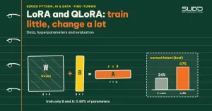
LoRA (Low-Rank Adaptation) is a technique for fine-tuning large language models without updating the original weights: you freeze the matrix W, learn only two low-rank matrices B and A, and the layer output becomes Wx + (alpha/r)·BAx. The original paper by Hu et al. (2021) reports roughly a 10,000x reduction in trainable parameters compared with full fine-tuning of GPT-3 175B, with no added inference latency.
This article does not stop at theory. We trained a real LoRA adapter for the Qwen/Qwen2-0.5B model on an Apple M4 CPU (16 GB), on a business-style task: turning customer messages into JSON {"intent", "order_id"}. It has a baseline, three rank levels, a measurement of "forgetting" and an adapter merge, and every number is real output (code in code/s7-44; Python 3.12, torch==2.8.0, transformers==4.56.0, peft==0.17.0). QLoRA needs an NVIDIA GPU, so we state clearly which part was not run in this article. It follows Fine-tuning PhoBERT with Hugging Face for Vietnamese sentiment analysis (full fine-tuning of a small model) and Running a local LLM with Ollama and llama.cpp: model choice, quantization and performance.
When to fine-tune with LoRA
Try the cheaper options first: prompts with worked examples, structured output, then RAG if knowledge is missing. Fine-tuning fits when you need the model to behave consistently (format, tone, internal labels) or want a small model to replace a large one. Do not use it to load knowledge that changes daily, such as prices or stock levels.
How LoRA works
A linear layer in a Transformer has a weight matrix W of size d_out × d_in. Full fine-tuning learns a ΔW of the same size as W. The hypothesis in the LoRA paper is that the change needed to adapt to a task has a low "intrinsic rank", so you can write ΔW = B·A with B of size d_out × r, A of size r × d_in and a small r. The parameter count of a layer drops from d_out·d_in to r·(d_in + d_out). Initializing B = 0 means the model starts out identical to the original; the added output is multiplied by the factor alpha/r.
| LoraConfig parameter | Meaning | Practical notes |
|---|---|---|
r | Rank of B·A, which sets the learning capacity | 8–16 is a reasonable starting point; increase it when the model underfits |
lora_alpha | Scaling factor, effective scale = alpha/r | Keep the alpha/r ratio fixed; alpha = r or 2r is common |
lora_dropout | Dropout on the LoRA branch | Helps when data is scarce |
target_modules | Which layers get LoRA | "all-linear" attaches to every linear layer (except the output layer), as in the QLoRA setup |
use_rslora | Changes the scale to alpha/√r | More stable at high rank |
use_dora | Separates weight magnitude and direction | Costs extra compared with plain LoRA |
The two variants in the table have clear sources. rsLoRA (Kalajdzievski, 2023) shows the adapter should be divided by the square root of the rank rather than the rank itself, because the old scaling slows learning at large ranks. DoRA (Liu et al., 2024) uses LoRA only to update the direction of the weights and learns the magnitude separately.
The task and data for LoRA
The data is simulated customer messages for 6 intents: tra_cuu (order lookup), huy_don (cancel order), doi_dia_chi (change address), xuat_hoa_don (issue invoice), khieu_nai (complaint), khac (other). Order IDs look like DH-xxxx; "other" messages have no order ID, so order_id is null. The key point: the training set and the test set use different sentence templates. Each intent has 6 templates to learn from and 3 entirely different templates for testing. For example, train on "Please cancel order {o}" while testing on "I'd like to withdraw {o}, I'm not buying it anymore". Mixing the same templates into both sets is data leakage (as discussed in the feature engineering article) and the score will look good for no real reason.
def make(split, n, seed):
    rng = random.Random(seed)
    names = list(INTENTS)
    rows = []
    for i in range(n):
        intent = names[i % len(names)]
        tpl = rng.choice(INTENTS[intent][split])      # split = "train" or "test"
        oid = None if intent == "khac" else f"DH-{rng.randint(1000, 9999)}"
        text = tpl.format(o=oid) if oid else tpl
        rows.append({"text": text,
                     "target": json.dumps({"intent": intent, "order_id": oid}, ensure_ascii=False)})
    rng.shuffle(rows)
    return rows
We used 240 training samples and 120 test samples, deliberately small because the machine only has a CPU. When reading the results, remember that the 120 test samples come from only 18 templates, so the measurement is noisy.
Baseline: what the base model can do before fine-tuning
Without a baseline you cannot tell how much fine-tuning is worth. We ran the base Qwen2-0.5B two ways: zero-shot (only "Message: … JSON:") and 3-shot (3 worked examples added to the prompt). Three metrics: json_hop_le (JSON parses), dung_intent (correct intent) and khop_hoan_toan (exact match: correct intent and order ID). Real output of baseline.py:
zero-shot {'json_hop_le': 0.058, 'dung_intent': 0.0, 'khop_hoan_toan': 0.0} | 924s
  example: 'Send an email for DH-7428' | correct: {"intent": "xuat_hoa_don", "order_id": "DH-7428"}
3-shot {'json_hop_le': 1.0, 'dung_intent': 0.242, 'khop_hoan_toan': 0.242} | 82s
  example: '{"intent": "khac", "order_id": null}' | correct: {"intent": "xuat_hoa_don", "order_id": "DH-7428"}
general NLL (base): 2.821
Zero-shot is almost useless (only 5.8% of outputs are valid JSON). 3-shot forces the format (100% valid JSON), but the 0.5-billion-parameter model picks the right intent only 24.2% of the time. The 924 seconds for the zero-shot run does not reflect model speed: the machine was busy, and the model generated up to 40 tokens per message because it did not know when to stop. The last line, general NLL, is a "forgetting" measurement explained in the evaluation section.
Training a LoRA adapter step by step
The configuration holds everything fixed except the rank, so the runs are comparable: 3 epochs, batch size 8, learning rate 2e-4 (a common value for LoRA, much higher than for full fine-tuning), lora_dropout=0.05, alpha = 2r, with LoRA attached to every linear layer:
cfg = LoraConfig(r=r, lora_alpha=alpha, lora_dropout=0.05,
                 target_modules="all-linear", task_type="CAUSAL_LM")
model = get_peft_model(base, cfg)
trainable, total = model.get_nb_trainable_parameters()
The easiest thing to get wrong when fine-tuning a text-generation model is what the loss is computed on. We want the model to learn only the answer (the JSON), not to relearn "generating" the customer's message. So we set the label to -100 (ignored by the loss) for the prompt part, and add an end-of-sequence token eos after the JSON so the model knows when to stop:
def encode(row):
    p = tok(PROMPT.format(text=row["text"]))["input_ids"]
    t = tok(" " + row["target"] + tok.eos_token)["input_ids"]
    return p + t, [-100] * len(p) + t          # loss only on the JSON answer
Running python train_lora.py 8 gives this real output (warning lines trimmed):
r=8 alpha=16: trainable 4,399,104 / 498,431,872 = 0.88%
epoch 1 step 1/90 loss 3.1850
epoch 1 step 10/90 loss 0.4431
epoch 1 step 20/90 loss 0.0486
epoch 1 step 30/90 loss 0.0019
epoch 3 step 90/90 loss 0.0001
training: 239s
test (zero-shot prompt, fine-tuned): {'json_hop_le': 1.0, 'dung_intent': 0.467, 'khop_hoan_toan': 0.467}
adapter size: 17.6 MB
Only 0.88% of parameters are trained and the adapter weighs 17.6 MB, while the base model is over 1 GB in float32. The number 4,399,104 can be verified with the formula r·(d_in + d_out): Qwen2-0.5B has 24 layers, hidden size 896, MLP size 4864, and K/V only 128 wide (grouped-query attention), so each layer has 8·(1792 + 1024 + 1024 + 1792) + 3·8·(896 + 4864) = 183,296 parameters, and 24 layers give exactly 4,399,104.
Reading the results: how much rank is enough
We reran with r = 2 and r = 32, using the same seed and data:
| Configuration | Trainable parameters | Correct intent (test) | NLL, ordinary sentences | Adapter |
|---|---|---|---|---|
| Base, 3-shot | 0 | 24.2% | 2.821 | none |
| LoRA r=2, alpha=4 | 1,099,776 (0.22%) | 53.3% | 2.765 | 4.4 MB |
| LoRA r=8, alpha=16 | 4,399,104 (0.88%) | 46.7% | 3.470 | 17.6 MB |
| LoRA r=32, alpha=64 | 17,596,416 (3.44%) | 55.0% | 4.000 | 70.4 MB |
Read honestly, the results say three things and cannot say one. First, LoRA is worth it: all three ranks nearly double the 3-shot baseline (24.2% up to 47–55%) and give 100% valid JSON without any examples in the prompt, which means a shorter prompt.
Second, the model is not good enough for production: about half of the messages still get the wrong intent. Third, the training loss drops to nearly 0 after 30–60 steps depending on rank (r=8 and r=32 after 30 steps, r=2 more slowly) while the test score is only 47–55%, a sign that the model memorized the 36 templates rather than generalizing.
What we cannot conclude: which rank is best. The differences of 46.7%, 53.3% and 55.0% fall within the error of a measurement on 120 samples from 18 templates and a single seed (the standard deviation is roughly √(0.5·0.5/120) ≈ 4.6 percentage points, and that is an underestimate because the samples are not independent). Choosing a rank requires a larger test set and multiple seeds.
The remaining errors point to something interesting. On the first sample the model returned "intent": "xuat_nai", a label that does not exist, because the model generates token by token freely and can splice a label incorrectly. For a closed-label problem, enforce the labels with constrained decoding or validate with a schema as in extracting data with an LLM and Pydantic, rather than trusting fine-tuning alone.
Evaluation: measure what was learned and what was forgotten
Evaluating a fine-tune needs at least three layers. Layer one is the target task on unseen data, as above. Layer two is general ability: does the model forget what it knew? We used a simple, cheap measure, the NLL (negative log-likelihood per token) of 5 ordinary Vietnamese sentences, lower is better, compared before and after. The results: base 2.821; r=2 gives 2.765; r=8 gives 3.470; r=32 gives 4.000. The trend suggests (observed on 1 seed, 3 ranks, 5 sentences) that the higher the rank, the worse the model does on ordinary sentences. Rank is not the only factor, since a training loss near 0 and a fixed alpha/r ratio also push the model away from the original.
With 5 sentences this is only a rough indicator; a serious version needs a large enough general evaluation set (knowledge, reasoning, safety). The fact that 2.765 is lower than 2.821 does not mean r=2 is "better than the base"; it is within noise.
This direction matches the study "LoRA Learns Less and Forgets Less" (Biderman et al., 2024): with typical low-rank settings, LoRA learns less than full fine-tuning on coding and math, but retains out-of-domain ability better. In other words, LoRA is a trade-off, not a free shortcut. Layer three is evaluation on real outputs: read the wrong samples by hand. For free-form generated text you also need test suites and an LLM as judge, the topic of the next article.
Merging the LoRA adapter and deploying
At inference time the adapter can be kept separate (swapping adapters per customer on the same base model) or merged into the weights with merge_and_unload() so the model runs like an ordinary model. This function merges the LoRA weights into the base model, removes the LoRA layers and returns the merged base model, so you need to reassign: model = model.merge_and_unload(). Verify with merge_check.py, real output:
total parameters: 498,431,872 (adapter not merged) -> 494,032,768 (merged)
identical outputs: 40/40
time for 40 messages: 6.0s (separate adapter) vs 5.3s (merged)
exact match (merged): {'json_hop_le': 1.0, 'dung_intent': 0.475, 'khop_hoan_toan': 0.475}
The difference between the two parameter lines, 4,399,104, is exactly the number of adapter parameters absorbed into the model; the outputs are identical on all 40 messages, and the merged model is slightly faster (5.3 seconds versus 6.0 seconds, on a machine running many tasks, so treat them as the same order of magnitude). The score of 0.475 on 40 messages differs from 0.467 on 120 messages because the sample size differs, one more example of measurement noise.
On licensing: the Qwen/Qwen2-0.5B model card on Hugging Face lists the Apache-2.0 license at the time of writing, so you can reuse the adapter, but check the model card of the base model you choose before deploying. The data in this article is simulated data written by Sudo, and contains no real customer data.
QLoRA: LoRA on a 4-bit quantized model
The main limit of LoRA on large models is the memory for the original weights, since we still have to load them. QLoRA (Dettmers et al., 2023) solves this by quantizing the base model to 4-bit, freezing it, and backpropagating gradients through it into the LoRA adapters. The paper proposes three techniques: the 4-bit NormalFloat (NF4) data type, double quantization (quantizing the quantization constants as well) and paged optimizers (handling memory spikes); with them, a 65-billion-parameter model can be fine-tuned on a single 48 GB GPU. An illustrative configuration (using the BitsAndBytesConfig and prepare_model_for_kbit_training classes from Transformers and PEFT) looks like this:
bnb_config = BitsAndBytesConfig(
    load_in_4bit=True,
    bnb_4bit_quant_type="nf4",
    bnb_4bit_compute_dtype=torch.bfloat16,
    bnb_4bit_use_double_quant=True,
)
model = AutoModelForCausalLM.from_pretrained(name, quantization_config=bnb_config, device_map="auto")
model = prepare_model_for_kbit_training(model)
model = get_peft_model(model, LoraConfig(r=16, lora_alpha=16, lora_dropout=0.1,
                                          target_modules="all-linear", task_type="CAUSAL_LM"))
This snippet needs an NVIDIA GPU (the bitsandbytes library) and was not run in this article: our test machine is an Apple M4 without an NVIDIA GPU, so we do not present QLoRA numbers as if they had been measured. Instead, memory_estimate.py calculates (does not measure) the weight memory for a Llama-style 7-billion-parameter model and the matching number of LoRA parameters:
7B weights (6.74 billion parameters):
  16-bit    :  12.6 GiB
  8-bit     :   6.3 GiB
  4-bit NF4 :   3.1 GiB
LoRA parameters when attached to all 7 linear matrices per layer:
  r=8  :   20.0 million = 0.30% | Adam fp32 (16 bytes/parameter: weights, gradient, 2 moments) ~0.30 GiB
  r=16 :   40.0 million = 0.59% | Adam fp32 (16 bytes/parameter: weights, gradient, 2 moments) ~0.60 GiB
  r=64 :  159.9 million = 2.37% | Adam fp32 (16 bytes/parameter: weights, gradient, 2 moments) ~2.38 GiB
This is the memory for the weights alone plus the adapter's optimizer state; activations, sequence length and batch size add more, so do not read these numbers as the total GPU requirement. The takeaway is the ratio: 4-bit weights are only about a quarter of the 16-bit version, and the trainable part (adapter plus optimizer) is much smaller than in full fine-tuning, which must hold gradients and two moments for all 6.74 billion parameters. In return, quantization costs a little accuracy, and according to the PEFT documentation, merging an adapter into a quantized model requantizes the weights, so they can no longer be separated exactly as before.
Choosing LoRA parameters: a practical guide
- Start with r = 8 or 16 and
target_modules="all-linear". Attaching only to q and v saves more but usually learns less; the QLoRA setup attaches to every linear layer. - Set alpha at a fixed ratio to r (
alpha = ror2r) and tune the learning rate first, then r. If you use a large rank, tryuse_rslora=Trueso the scaling does not slow learning. - Few epochs, and watch the test set. A training loss falling to 0 does not mean good; stop early when the test score stops improving.
- Clean, varied, label-balanced data is worth far more than many repeated samples; record the base model version, seed and configuration alongside the adapter.
Common mistakes
- Loss computed on the prompt too: the model wastes capacity learning to "imitate" the question. Use the label
-100for the prompt part. - Forgetting the end token: the model does not know when to stop and generates garbage after the JSON (we cut at the first line when scoring, but in production this must be handled properly).
- Leakage between train and test: duplicate templates or the same customer in both sets inflate the score.
- Drawing conclusions from a small test set: as we saw, a difference of a few percentage points on 120 samples is not enough to pick a configuration.
- Putting real personal data into the training set: the model may memorize it and repeat it back. Anonymize first, and use simulated data when experimenting, as in this article.
LoRA fine-tuning checklist
- You have a baseline (prompt or few-shot) to compare against, not just zero-shot.
- The test set uses different sentence templates and different users than the training set, and is large enough to tell configurations apart.
- Loss is computed only on the answer part, with an end token.
- Measure both the target task and forgetting on a general set.
- Read the wrong samples by hand; for closed-label outputs, validate with a schema.
- Anything that needs a GPU and was not run is stated clearly, with no numbers inferred.
Setup (requirements.txt pins only the direct packages; every script limits itself to 2 CPU threads with torch.set_num_threads(2) in common.py, so running alongside other processes does not hog the CPU): python3.12 -m venv .venv && .venv/bin/pip install -r requirements.txt, then run baseline.py, train_lora.py 8 (change the argument to 2 or 32 to repeat the rank table), merge_check.py and memory_estimate.py in code/s7-44; the *_output.txt files are the output pasted above. Primary sources: the PEFT LoRA guide, and the LoRA and QLoRA papers. To understand the architecture LoRA attaches to, reread Transformer and attention: understanding the architecture through code.
Next article
LLM evaluation and guardrails: test suites, LLM-as-judge and prompt injection defense. Fine-tuning is only half the job: the next article builds an automated test suite for model output, uses an LLM as a controlled judge and blocks prompt injection before anything reaches production.