Almost every language model you hear about today, from BERT and PhoBERT to text-generation models, is built on the same architecture: the Transformer. This article does not argue which model is "smarter". It opens up the architecture itself. We implement the attention mechanism in PyTorch, check every number against the standard library, build a small Transformer that learns to sort digits, and then read the attention matrices of the real PhoBERT model on a Vietnamese sentence. By the end, you should be able to look at a Transformer model and say what each block does, how many parameters it costs, and why long sequences are expensive.
The article builds on basic PyTorch from PyTorch basics: tensors, autograd and the training loop and on word representations from Word embeddings: Word2Vec, FastText and representing word meaning. The output below is real, run on the CPU of an Apple Silicon machine with PyTorch 2.2.2 (released 03/2024); the PhoBERT part uses transformers 4.38.2 and pyvi 0.1.1. The APIs used here (nn.MultiheadAttention, F.scaled_dot_product_attention) have existed since PyTorch 2.0. Because PyTorch versions and hardware differ, a rerun may differ by a few thousandths in accuracy and a few percent in individual attention cells; the conclusions do not change.
Why we need the Transformer: the limits of RNNs
Before the Transformer arrived in 2017, the dominant sequence models were recurrent networks (RNN, LSTM): they read one token at a time and gather information into a single hidden state. Their limits are clear: token 100 can only be computed after token 99, so they are hard to parallelize, and information from the first token must pass through a hundred steps to reach the last one, so it tends to fade.
The paper Attention Is All You Need by Vaswani et al. (2017) dropped recurrence and convolution entirely and used only the attention mechanism. According to its abstract, the model reached 28.4 BLEU on the WMT 2014 English-to-German translation task, more than 2 BLEU above the best previous results (including ensembles), and 41.8 BLEU on English-to-French after 3.5 days of training on eight GPUs, at a small fraction of the training cost of the best contemporary models. The key point: all positions are processed in parallel, and any two tokens are connected directly in a single step.
Attention in the Transformer: the Q, K and V matrices
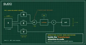
For each token, the model produces three vectors through three learned matrix multiplications: query Q ("what information do I need"), key K ("what information do I hold") and value V ("the content I hand over"). The compatibility between token i and token j is the dot product of Qi with Kj; softmax turns a row of scores into weights that sum to 1; the output for token i is the weighted sum of the V vectors. The formula in the paper is Attention(Q,K,V) = softmax(QK^T / sqrt(d_k)) V. The implementation (attention.py):
def scaled_dot_product_attention(q, k, v, mask=None):
    d_k = q.size(-1)
    scores = q @ k.transpose(-2, -1) / math.sqrt(d_k)
    if mask is not None:
        scores = scores.masked_fill(~mask, float("-inf"))
    w = torch.softmax(scores, dim=-1)
    return w @ v, w
Running the Transformer attention block on four tokens with d=3 (using the input vectors themselves as Q, K and V so the numbers stay readable):
weights (each row sums to 1):
 tensor([[0.320, 0.180, 0.320, 0.180],
        [0.180, 0.320, 0.320, 0.180],
        [0.230, 0.230, 0.410, 0.129],
        [0.209, 0.209, 0.209, 0.373]])
row sums: tensor([1.000, 1.000, 1.000, 1.000])
The third token [1,1,0] resembles both the first and the second, so it attends equally (0.23) to both and 0.41 to itself. The fourth token [0,0,1] is orthogonal to the other three, so all its scores against them are 0, and the weights fall evenly at 0.209.
Why we divide by the square root of d_k
If the components of q and k are independent with mean 0 and variance 1, the dot product q·k has variance d_k, so its standard deviation is the square root of d_k. With a large d_k, big scores saturate the softmax: one element takes almost all the weight and the gradient to the other elements is close to 0. Measured with d_k = 64:
std(q.k)=8.00 (≈ sqrt(64)=8)   std(q.k/sqrt(d))=1.00
softmax without scaling: mean max weight = 0.687 | with scaling: 0.096
Without scaling, the largest of 64 elements takes 68.7% of the weight on average; after scaling it takes only 9.6%, so attention stays "spread out" and can learn.
Multi-head attention in the Transformer: several points of view
A single attention head gives only one kind of mixing. Multi-head attention splits the d_model dimension into h parts; each head has its own Q, K and V projections with d_k = d_model / h, runs attention in parallel, then concatenates the results and multiplies by an output matrix WO. Each head can track a different relationship. The implementation:
class MultiHeadAttention(nn.Module):
    def __init__(self, d_model, n_heads):
        super().__init__()
        self.h, self.d_k = n_heads, d_model // n_heads
        self.wq, self.wk, self.wv = (nn.Linear(d_model, d_model) for _ in range(3))
        self.wo = nn.Linear(d_model, d_model)

    def split(self, x):  # (B,T,D) -> (B,h,T,d_k)
        B, T, _ = x.shape
        return x.view(B, T, self.h, self.d_k).transpose(1, 2)

    def forward(self, x, mask=None):
        q, k, v = self.split(self.wq(x)), self.split(self.wk(x)), self.split(self.wv(x))
        out, w = scaled_dot_product_attention(q, k, v, mask)
        B, _, T, _ = out.shape
        return self.wo(out.transpose(1, 2).reshape(B, T, -1)), w
Implementing a Transformer by hand is easy to get wrong, so we verify it. Copy the same weights into torch.nn.MultiheadAttention and into F.scaled_dot_product_attention, then compare the results:
max output difference: 8.94e-08 | weights: 5.96e-08
vs F.scaled_dot_product_attention: 7.45e-08
A difference around 1e-7 is float32 rounding error, so the hand-written code matches the library. In practice, call the standard function: according to the PyTorch documentation, scaled_dot_product_attention automatically chooses between FlashAttention-2, memory-efficient attention and a C++ implementation depending on the input, and accepts attn_mask or is_causal (using both at once raises an error).
The causal mask: a text-generating Transformer cannot "peek"
When generating text one token at a time, token i must not see the tokens after it, otherwise training becomes cheating. The way to do this is to set the scores at positions j greater than i to negative infinity before the softmax, so the weights are exactly 0:
tensor([[1.000, 0.000, 0.000, 0.000, 0.000],
        [0.017, 0.983, 0.000, 0.000, 0.000],
        [0.033, 0.064, 0.903, 0.000, 0.000],
        [0.210, 0.151, 0.169, 0.471, 0.000],
        [0.012, 0.054, 0.063, 0.005, 0.866]])
This is the difference between the two families of Transformers: BERT and PhoBERT are bidirectional encoders (no mask, every token sees the whole sentence), while GPT-style text-generation models are decoders that use a causal mask.
Positional encoding: the Transformer needs to know order
Attention is a weighted mixing operation, so it has no notion of "comes before" or "comes after". We can demonstrate this: randomly permute the input tokens, then apply the inverse permutation to the output, and the result must be identical if attention is permutation equivariant (changing the input order changes the output order accordingly, with no information about position):
permute input then un-permute output gives identical result: True
after adding sinusoidal position, still permutation equivariant? False
That is why a Transformer must be given positions. The original paper adds to the embedding a sin/cos vector with a different frequency in each dimension: PE(pos,2i)=sin(pos/10000^(2i/d)), PE(pos,2i+1)=cos(...). Position 0 gives [0, 1, 0, 1, ...], position 1 gives [0.841, 0.54, 0.533, 0.846, 0.311, 0.95] in the first six dimensions: the same pattern, shifted in phase. After adding this vector, permuting the input changes the output (the False on the second line), which means the model can now tell order apart. Many other models use learned positions, but the principle is the same: positions must be injected from outside.
Building a small Transformer: learning to sort 8 digits
A Transformer encoder block consists of multi-head attention, a two-layer feed-forward network (expand 4x, then project back), two LayerNorm layers and two skip connections. We use the pre-LN form: normalize before each branch, which usually makes training more stable than the post-LN form of the original paper (analyzed in On Layer Normalization in the Transformer Architecture, Xiong et al., 2020). The code (mini_transformer.py):
class Block(nn.Module):
    def __init__(self):
        super().__init__()
        self.attn = MultiHeadAttention(D, H)
        self.ln1, self.ln2 = nn.LayerNorm(D), nn.LayerNorm(D)
        self.ff = nn.Sequential(nn.Linear(D, 4 * D), nn.GELU(), nn.Linear(4 * D, D))

    def forward(self, x):
        a, w = self.attn(self.ln1(x))
        x = x + a
        return x + self.ff(self.ln2(x)), w
The task: take 8 random digits from 0 to 9 and return them sorted. The model has 2 layers, d=64, 4 heads and 101,258 parameters, trained for 1,500 steps with batch size 128; comparing elements with each other is exactly what attention is good at. We run two versions of the Transformer: with and without positional encoding.
  [pos=True] step    0 loss=9.5350
  [pos=True] step  500 loss=0.1120
  [pos=True] step 1000 loss=0.0210
  [pos=True] step 1499 loss=0.0079
  => pos=True: per-position accuracy 0.998 | whole-sequence accuracy 0.988 | 101258 parameters | 15s
  [pos=False] step    0 loss=9.4835
  [pos=False] step  500 loss=1.7063
  [pos=False] step 1000 loss=1.6927
  [pos=False] step 1499 loss=1.6838
  => pos=False: per-position accuracy 0.301 | whole-sequence accuracy 0.000 | 101258 parameters | 15s
On 5,000 new sequences, the Transformer with positions gets the entire sequence right 98.8% of the time after 15 seconds of CPU training; the version without positions is stuck at a loss of 1.68 and gets 0% of whole sequences right. The cause is not missing parameters (both have 101,258) but the permutation equivariance shown above: each output position needs to know "which smallest element am I".
Reading the attention matrix of the trained Transformer
For the input [7, 2, 9, 2, 5, 0, 8, 3], the model returns exactly [0, 2, 2, 3, 5, 7, 8, 9]. The layer 2 attention matrix, averaged over 4 heads (rows are output positions, columns are input positions):
tensor([[0.00, 0.18, 0.00, 0.20, 0.01, 0.32, 0.00, 0.28],
        [0.00, 0.26, 0.02, 0.29, 0.01, 0.10, 0.00, 0.31],
        [0.02, 0.21, 0.01, 0.21, 0.15, 0.03, 0.02, 0.35],
        [0.05, 0.12, 0.00, 0.13, 0.27, 0.00, 0.02, 0.40],
        [0.17, 0.08, 0.01, 0.08, 0.46, 0.01, 0.05, 0.13],
        [0.53, 0.01, 0.01, 0.01, 0.23, 0.00, 0.14, 0.06],
        [0.52, 0.00, 0.07, 0.00, 0.02, 0.00, 0.36, 0.01],
        [0.50, 0.00, 0.24, 0.00, 0.00, 0.00, 0.26, 0.00]])
Part of the structure is readable. Row 4 (the output should be 5) puts 0.46 on column 4, where the input is indeed 5. Row 5 (needs 7) puts 0.53 on column 0, where the input is 7; row 6 (needs 8) attends to column 0 and column 6 (value 8); row 7 (needs 9) spreads over columns 0, 2 (value 9) and 6. The first four rows (needing 0, 2, 2, 3) concentrate on columns 1, 3, 5, 7, which hold exactly those small numbers. Do not over-read it: this is an average of four heads, not a clean sorting algorithm. The paper Attention is not Explanation (Jain and Wallace, 2019) warns that attention weights do not always explain a prediction, so treat this matrix as a clue for testing hypotheses, not as proof.
The quadratic cost of the Transformer in sequence length
The score matrix has size T x T for each head, so memory and time grow with the square of the sequence length. Measuring one Transformer attention layer (d=64, 4 heads, batch=1) on CPU:
T=  256  score matrix      1.0 MB (float32, 4 heads)  time     0.3 ms
T=  512  score matrix      4.2 MB (float32, 4 heads)  time     1.1 ms
T= 1024  score matrix     16.8 MB (float32, 4 heads)  time     3.9 ms
T= 2048  score matrix     67.1 MB (float32, 4 heads)  time    12.7 ms
T= 4096  score matrix    268.4 MB (float32, 4 heads)  time    45.5 ms
Each time T doubles, the score matrix memory grows exactly 4x and the time grows about 3.5 to 4x (from 12.7 to 45.5 ms in the last two rows). These figures are for one layer and one sequence; multiply by the number of layers and the batch size and you run out of RAM very quickly. That is why FlashAttention (Dao et al., 2022) was created: it computes exact attention but works in blocks to reduce GPU memory reads and writes, and reports a 3x speedup on GPT-2 with 1,000-token sequences.
PhoBERT is a real Transformer: where the parameters live
Finally, let us check what we just built against a real model. PhoBERT (Dat Quoc Nguyen and Anh Tuan Nguyen, 2020) is a pre-trained language model for Vietnamese that achieved state-of-the-art results on several Vietnamese tasks when it was published. Reading its configuration with transformers (phobert_attention.py):
layers=12 | heads=12 | d_model=768 | d_k=64 | d_ff=3072 | max_pos=258
total parameters: 135.0 million
  embedding 49.4 million (37%), 12 encoder blocks 85.1 million
  one block: attention 2.36 million | feed-forward 4.72 million
Compared with the base version of the original Transformer (6 layers, d_model 512, 8 heads, d_ff 2048), PhoBERT-base is twice as deep and wider, but d_k is still 64: 768/12. Two takeaways. First, the feed-forward network has twice the parameters of attention in each block (4.72 versus 2.36 million), so attention alone does not make the model. Second, 37% of the parameters sit in the embedding table for the 64,001-token vocabulary.
PhoBERT attention on a Vietnamese sentence
The test sentence is "Giảng viên giải thích rất dễ hiểu nhưng phòng học quá nóng" (roughly, "The instructor explained things very clearly, but the classroom was too hot"). PhoBERT requires word-segmented input, so we use pyvi to join the syllables of compound words with underscores:
tokens: ['<s>', 'Giảng_viên', 'giải_thích', 'rất', 'dễ', 'hiểu', 'nhưng', 'phòng', 'học', 'quá', 'nóng', '</s>']
attention shape (layer, head, T, T): (12, 12, 12, 12) | each row sums to 1.0
This is a tensor of 12 layers x 12 heads, each head a 12 x 12 matrix like the one we implemented, with every row summing to 1. Asking where the token "nóng" ("hot") attends most in a few different heads:
  layer  1 head  1: nóng:0.34, <s>:0.23, rất:0.07
  layer  1 head  6: Giảng_viên:0.41, hiểu:0.10, phòng:0.07
  layer  6 head  4: nóng:0.29, <s>:0.29, </s>:0.12
  layer  9 head  8: </s>:0.91, quá:0.04, <s>:0.03
  layer 12 head  1: nóng:0.48, <s>:0.25, </s>:0.13
  layer 12 head 10: </s>:0.51, <s>:0.46, phòng:0.01
The heads behave very differently: layer 1 head 1 looks at itself, layer 1 head 6 looks far away to "Giảng_viên", and layer 9 head 8 puts 91% on the end-of-sentence token. This matches the findings of What Does BERT Look At? (Clark et al., 2019): many BERT heads focus on the separator token, some follow a fixed positional offset, and some spread broadly. Aggregate numbers for this sentence:
Mean attention entropy (nats) by layer (max = ln T = 2.48):
   [1.85, 1.02, 1.27, 1.51, 1.41, 1.63, 1.58, 1.33, 0.97, 0.99, 1.01, 1.17]
Share of attention going to the <s> token, mean by layer:
   [0.2, 0.55, 0.31, 0.3, 0.31, 0.35, 0.17, 0.04, 0.05, 0.05, 0.05, 0.32]
Entropy measures how spread out attention is: the maximum is 2.48 nats if attention is perfectly uniform over the 12 tokens. Layer 1 is the most spread out (1.85), and layers 9 and 10 are the most focused (0.97 and 0.99). In layer 2, on average 55% of attention goes to the first token, which suggests the model uses this token as a "parking spot" when a head has nothing to retrieve. This is the result on one sentence: illustration only, and a real conclusion would need measurements over thousands of sentences.
When not to use a Transformer
- Tabular data with a few thousand rows: gradient boosting as in Gradient boosting with XGBoost and LightGBM: when it beats deep learning usually wins and is far cheaper.
- Very long sequences on small hardware: the Transformer uses quadratic memory (see the measurements above), so you need FlashAttention, sliding windows or a different architecture.
- Simple text classification: TF-IDF with a linear model is usually enough as a baseline; a Transformer is only worth it when the baseline is truly lacking.
Common mistakes when implementing a Transformer yourself
- Forgetting to divide by the square root of d_k: the softmax saturates and the loss is hard to reduce; the experiment above shows a largest weight of 0.687 versus 0.096.
- Applying the mask along the wrong axis: using
masked_fillwith an inverted mask, or a mask on the query axis instead of the key axis, lets the model peek at the future while the loss still looks great. - Mixing up shapes when splitting heads: forgetting
transposeor usingreshapein the wrong order mixes tokens across heads; always compare againstnn.MultiheadAttentionas in this article. - No position information: the model runs normally but is blind to order, exactly like the
pos=Falseversion above.
Checklist for understanding a Transformer model
- For every Transformer, know d_model, the number of layers, the number of heads, d_k = d_model / number of heads, and d_ff; you can read them from the config file.
- Tell the Transformer encoder (bidirectional, like BERT/PhoBERT) apart from the decoder (causal mask, generates text).
- Know that positions are injected from outside; verify with a permutation experiment.
- Use
F.scaled_dot_product_attentionin real code; implement it yourself only to learn the Transformer.
The code is in code/s7-27: attention.py, mini_transformer.py, phobert_attention.py, plus the *_output.txt files and requirements.txt. phobert_attention.py needs the vinai/phobert-base model and pyvi. The numbers are real output but cover only one sentence and one random seed, so use them to illustrate the mechanism.
Next article
Fine-tuning PhoBERT with Hugging Face for Vietnamese sentiment analysis. Now that you understand the Transformer architecture inside, the next article adds a classification head on top of PhoBERT, fine-tunes it on Vietnamese review data and measures the result against a TF-IDF baseline.