After Embeddings and semantic search: sentence-transformers and FAISS, every project hits the same next question: where do the vectors live once the data grows, gets edited, gets deleted and has to be filtered by store or by category? A vector database is more than a nearest-neighbor index; it also handles durable storage, updates, attribute filtering, concurrent access and backups.
This article puts three popular vector database options on the same dataset: FAISS (a library), pgvector (a PostgreSQL extension) and Qdrant (a dedicated server). All three use the HNSW algorithm, so the differences lie in everything around the algorithm. Every number was measured by us on an Apple M4 and pasted verbatim from the output files.
What a vector database solves that a NumPy array does not
In the previous article, 48 FAQ entries sat in a NumPy array, and scanning all of them still answered in the blink of an eye. The problem changes when vectors reach the millions and many people write and read at the same time. A vector database needs approximate nearest neighbor (ANN) search, durable storage, deleting and updating single records, metadata filtering, concurrent access with permissions, replication and backups.
The three vector database candidates sit in three different places. FAISS (Meta) is a library that runs inside your own process; it is very fast, but you have to write most of the capabilities above yourself. pgvector adds a vector type and two index types to PostgreSQL, so it inherits transactions, backups, permissions and SQL. Qdrant is a server written in Rust, built for vectors with payloads, and it talks over REST or gRPC.
HNSW: the algorithm shared by every vector database
HNSW (Hierarchical Navigable Small World) was proposed by Malkov and Yashunin in 2016. It is the most widely used index and appears in all three systems compared in this article. Each vector is randomly assigned a top layer following an exponentially decaying distribution, so the upper layers are very sparse while the bottom layer holds every point. When searching, the algorithm enters at the top layer, jumps far to the region near the query, then descends through the denser layers, much like a skip list, which gives roughly logarithmic complexity in the number of vectors.
| Meaning | FAISS | pgvector | Qdrant |
|---|---|---|---|
| Maximum links per node | M | m (default 16) | m |
| Search width while building the graph | efConstruction | ef_construction (default 64) | ef_construct |
| Search width at query time | efSearch | hnsw.ef_search (default 40) | hnsw_ef |
The defaults come from the pgvector documentation. Larger m and ef_construction give a better graph but build more slowly and use more memory; a larger ef_search gives higher recall but makes every query slower. It is the most important knob, and you can change it per query or per session without rebuilding the index.
The dataset and how we measure each vector database
For a fair comparison we use the fashion-mnist-784-euclidean set from ANN-Benchmarks: 60,000 vectors of 784 dimensions, L2 distance, with ground-truth neighbors. We take 1,000 queries and measure recall@10: of the 10 results returned, how many are among the 10 true neighbors. Environment: PostgreSQL 17 with pgvector 0.8.0 (image pgvector/pgvector:0.8.0-pg17) and Qdrant 1.12.4 running in Docker, and FAISS 1.9.0 inside the Python process:
docker run -d --name pgv -e POSTGRES_PASSWORD="$PG_LOCAL_PASSWORD" -p 5433:5432 pgvector/pgvector:0.8.0-pg17
docker run -d --name qdr -p 6333:6333 qdrant/qdrant:v1.12.4
Limits of the measurement: queries are issued sequentially from a single thread; FAISS runs in the same process, while pgvector and Qdrant also pay for the network and protocol. This is latency for one client, not the maximum throughput with many parallel connections, and you should not generalize it to your own data.
FAISS: the fastest vector database, but only a library
The bench_faiss.py script builds Flat, IVFFlat and HNSW indexes and sweeps the parameters. Real output (intermediate lines trimmed; the full version is in bench_faiss_output.txt):
index                               build (s)  recall     QPS  p50 ms  p99 ms
Flat (full scan)                       0.47   1.000     145    6.16   17.89
IVFFlat nlist=256 nprobe=4             0.66   0.945    6666    0.12    0.41
IVFFlat nlist=256 nprobe=16            0.66   0.999    1907    0.44    1.82
HNSW M=16 efC=200 efSearch=10         57.30   0.939    7989    0.08    0.36
HNSW M=16 efC=200 efSearch=50         57.30   0.997    7115    0.13    0.26
HNSW M=16 efC=200 efSearch=200        57.30   0.999    3384    0.29    0.45
The full scan gives recall 1.000 at 6 ms per query: at this scale the naive approach is still usable. HNSW reaches recall 0.997 at about 0.13 ms, roughly 47 times faster than Flat at p50, but it takes 57 seconds to build versus 0.47 seconds. IVFFlat builds in only 0.66 seconds and reaches 0.999 at nprobe=16, which is worth considering when the data rarely changes. QPS and p99 fluctuate between runs because the machine is shared with other tasks, so read the trend rather than individual rows.
The price of using FAISS as a vector database sits outside the table. update_delete.py tries deleting vectors from HNSW and from Flat wrapped in IndexIDMap2:
FAISS IndexHNSWFlat.remove_ids: error -> Error in virtual size_t faiss::Index::remove_ids(const IDSelector &) at ...
FAISS Flat+IDMap2, before delete, top-3: [42, 4160, 3464]
FAISS Flat+IDMap2, after remove_ids(42), top-3: [4160, 3464, 822] | ntotal = 4999
IndexHNSWFlat does not support deletion: the FAISS wiki states plainly that HNSW cannot remove vectors because that would break the graph. To delete, you either keep your own "deleted" list to filter the results or rebuild the index periodically. FAISS also has no authentication and no database-style attribute filtering. That is why it is not yet a complete vector database: it suits a static set loaded once (a nightly build, an experiment) better than the core of a service with continuous writes.
pgvector: a vector database inside PostgreSQL
With pgvector, a vector is just a column, and the index is created with familiar SQL:
CREATE EXTENSION IF NOT EXISTS vector;
CREATE TABLE items (id int PRIMARY KEY, embedding vector(784));
CREATE INDEX items_hnsw ON items USING hnsw (embedding vector_l2_ops)
  WITH (m = 16, ef_construction = 200);
SET hnsw.ef_search = 40;
SELECT id FROM items ORDER BY embedding <-> $1 LIMIT 10;
The <-> operator is L2 distance; <=> is cosine and <#> is negative inner product. Real output of bench_pgvector.py (trimmed):
loaded 60000 rows: 4.6s | PostgreSQL 17 | pgvector 0.8.0 | table 240 MB
index                               build (s)  size     recall     QPS  p50 ms  p99 ms
no index (sequential scan)              0.0        -   1.000       7  116.64  354.87
HNSW m=16 efC=200 ef_search=10         78.1   234 MB   0.972     733    1.05    5.15
HNSW m=16 efC=200 ef_search=40         78.1   234 MB   0.997     582    1.43    7.30
HNSW m=16 efC=200 ef_search=200        78.1   234 MB   0.999     180    4.37   24.22
IVFFlat lists=245 probes=4              6.4   236 MB   0.950     271    3.10   14.41
IVFFlat lists=245 probes=16             6.4   236 MB   0.999     114    7.73   26.17
The HNSW index brings a query down from 116 ms (scanning the whole table) to 1.4 ms with recall 0.997 at ef_search=40. That is about 10 times slower than in-process FAISS, mostly because of the network, the PostgreSQL protocol and the query planner, not the algorithm. In return, this vector database brings all of PostgreSQL with it; deleting and updating are plain SQL, with transactions:
pgvector, after DELETE id=42, top-3: [4160, 3464, 822]
pgvector, after UPDATE id=7 to the vector of 42, top-3: [7, 4160, 3464]
Two points call for caution. First, build time: 78 seconds for 60,000 vectors at ef_construction=200, and inserting new data costs extra as well. Second, according to the documentation, the vector type can only be indexed up to 2,000 dimensions; larger embeddings need halfvec or dimensionality reduction.
Qdrant: a dedicated vector database with payloads
Qdrant is a standalone server-style vector database; each point it stores consists of an id, a vector and a JSON payload. A background optimizer builds HNSW for segments that are large enough, so bench_qdrant.py waits for the collection to reach the green state before measuring. Real output (trimmed):
load + index build for 60000 points: 25.8s | segments=7 | indexed_vectors=59000
HNSW m=16 efC=200 hnsw_ef=10         0.987     169    4.71   25.53
HNSW m=16 efC=200 hnsw_ef=40         0.999     213    4.01   15.10
HNSW m=16 efC=200 hnsw_ef=200        1.000     192    4.43   18.12
exact=True (full scan, 100 queries)  1.000     103    7.58   36.73
Qdrant reaches high recall from hnsw_ef=20 and builds faster than the HNSW of FAISS (57 seconds, single thread) and of pgvector (78 seconds): 25.8 seconds including loading the data, thanks to building several segments in parallel. This is not compared against IVFFlat, which builds faster still.
The latency of about 4 ms for this vector database is higher than pgvector in our measurement; most of it comes from sending a 784-number vector as JSON over REST. gRPC usually reduces this cost, but we did not measure it, so we do not claim how much. The line indexed_vectors=59000 out of 60,000 points shows that one small segment has no HNSW yet and is scanned sequentially, which is by design. Delete and upsert give the same results as pgvector:
Qdrant, after delete id=42, top-3: [4160, 3464, 822]
Qdrant, after upsert id=7 to the vector of 42, top-3: [7, 4160, 3464]
Metadata filtering: where each vector database differs most
Real queries almost always carry a condition: tenant, category, in stock. Plain HNSW knows nothing about conditions, so each system handles them differently. bench_filter.py gives each vector the label id % 100 (synthetic data to measure the mechanism, not a real attribute) and queries only group 7, about 1% of the rows. The exact answer is computed with NumPy on the filtered set.
600 / 60000 vectors belong to group 7 (1.0%); 300 queries, k=10
configuration                                            avg results  recall  p50 ms  p99 ms
pgvector, default plan (planner picks sequential scan)       10.0   1.000    2.48    2.78
pgvector HNSW ef_search=40 iterative_scan=off                 0.3   0.035    0.62    0.88
pgvector HNSW ef_search=40 iterative_scan=relaxed_order      10.0   1.000    4.37    7.88
pgvector HNSW ef_search=40 iterative_scan=strict_order       10.0   0.998    4.53    7.81
Qdrant hnsw_ef=40 + payload index                            10.0   1.000    2.09    3.29
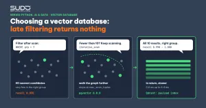
The second row is the subtlest failure of any vector database that uses an approximate index: when PostgreSQL is forced to use the HNSW index, it returns only 0.3 results on average instead of 10, with recall 0.035. The cause, according to the pgvector documentation: an approximate index applies WHERE after the scan. With ef_search=40, the index returns the 40 nearest candidates across the whole table and then discards the rows that are not in group 7; the group is only 1%, so very few remain. explain_filter.py shows this (trimmed):
--- force the index (enable_seqscan=off)
    Limit  (cost=1292.45..3329.38 rows=10 width=12)
      ->  Index Scan using items_hnsw on items  (cost=1292.45..125137.52 rows=608 width=12)
            Order By: (embedding <-> '[...]'::vector)
            Filter: (grp = 7)
iterative_scan=off: average results 0.35 | queries returning <10 rows: 300 | queries returning 0 rows: 210
iterative_scan=relaxed_order: average results 10.00 | queries returning <10 rows: 0 | queries returning 0 rows: 0
In off mode, 210 of 300 queries return 0 rows: the search feature looks normal but silently returns empty pages. With a 1% group, the planner picks a sequential scan on its own (correctly, since there are only 600 rows), so users do not hit the bug; it shows up when the condition is selective enough for the planner to choose the index, or when you force the index as we did.
pgvector 0.8.0 added iterative index scan (hnsw.iterative_scan): when there are not enough rows after filtering, the index keeps scanning until it has enough or reaches hnsw.max_scan_tuples (default 20,000). strict_order preserves exact distance order, while relaxed_order allows slight deviations for better recall. Both return the full 10 rows with recall 0.998 to 1.000; the price is latency of about 4.4 ms instead of 0.6 ms.
Qdrant takes a different approach: you create a payload index for the field you filter on. According to the Qdrant documentation, HNSW only gets filter-aware extra edges when it is built after the payload index exists, and the payload index also helps estimate cardinality to choose a search strategy. In the measurement, Qdrant returned the full 10 results, recall 1.000, p50 2.09 ms.
Note: bench_filter.py creates the payload index after loading the data, so our measurement makes exactly the mistake just described. The 1.000 figure reflects Qdrant's filtered query path, not yet an HNSW with filter edges; with a 1% group (600 points) the planner most likely scans directly through the payload index. We only measured the result, and we did not prove the internal mechanism. When evaluating a vector database with filtering, measure the number of results returned, not just latency.
Storage and memory of a vector database
The footprint.py script measures the same 60,000 vectors, with 179 MiB of raw data:
raw float32 data: 179 MiB
FAISS HNSW M=16      index file: 188 MiB
pgvector table items (heap + TOAST)       245 MB
pgvector index items_hnsw                 234 MB
Qdrant collection items on disk           235M
The pgvector HNSW index (234 MB) is larger than the raw data because it copies the vectors into index pages: the table plus the index is roughly double. FAISS HNSW adds only 9 MiB of graph because it keeps a single copy of the vectors. The Qdrant figure covers the whole collection directory (vectors, graph, payload). When a vector database grows to tens of millions of vectors, these factors decide server cost and are a reason to consider quantization; this article does not measure quantization.
Which vector database for which situation
| Situation | Try first | Reason |
|---|---|---|
| Static set, loaded once, running inside one service | FAISS | Fastest, no extra server |
| Already running PostgreSQL, a few million vectors or fewer | pgvector | Transactions, JOINs with the orders table, existing backups |
| Many tenants, complex filters, continuous writes | Qdrant | Payloads, in-index filtering, built-in replication and sharding |
| Need to delete exact individual records | pgvector or Qdrant | FAISS HNSW cannot delete single vectors |
A cautious rule for choosing a vector database: if you already operate PostgreSQL, start with pgvector and move to a separate vector database only when you measure a real bottleneck (latency, index size, write load, filtering features). Adding a system means adding monitoring, backups, upgrades and one more thing that can fail.
When you do not need a vector database
- Under a few tens of thousands of vectors (no vector database needed yet): a full scan with NumPy or
IndexFlatis fast enough (6 ms at 60,000 vectors, single thread) and 100% exact. - Queries are mostly keywords or product codes: BM25 or
LIKEis more accurate; consider hybrid search. - You must explain why a result appeared: vector distance is harder to explain than a keyword match.
Common mistakes when using a vector database
- Looking only at vector database latency and ignoring recall:
iterative_scan=offhas the lowest latency in the table but recall 0.035. - Comparing in-process FAISS with a service over the network and concluding which algorithm is faster: that compares architectures.
- A metric that does not match the index: an index built with
vector_l2_opscannot be used by a query that uses<=>. - Setting
ef_searchlower thank, or forgetting to adjust it after raisingk. - Creating the payload index after loading the data (Qdrant), or forgetting
ANALYZEafter a bulk load (PostgreSQL). - Building IVFFlat on an empty table: the centroids are chosen from the existing data, so quality is poor.
- Generalizing from a single configuration: the numbers in this article come from one dataset, one machine and one calling thread.
Vector database selection checklist
- Before choosing a vector database, count the current vectors and forecast 12 months out; record the dimensionality and the distance metric.
- Test each real filter condition at 1%, 10% and 50% selectivity; measure the number of results returned as well.
- Determine how often you delete and update; if you need to delete single records, rule out plain FAISS HNSW.
- Settle on an acceptable recall (usually 0.95 to 0.99) first, then choose
ef_search; measure p50 and p99. - Estimate storage and the time to rebuild the index when you change the embedding model.
- Check backup, restore and upgrades; measure with real data that has been anonymized.
The vector database comparison code is in code/s7-36: common.py, bench_faiss.py, bench_pgvector.py, bench_qdrant.py, bench_filter.py, explain_filter.py, update_delete.py, footprint.py and the *_output.txt files. The data is downloaded from ANN-Benchmarks (about 217 MB, not included in the code repository). Re-run it in the following order, inside code/s7-36:
python3.12 -m venv .venv && .venv/bin/pip install -r requirements.txt
mkdir -p data && curl -o data/fashion-mnist-784-euclidean.hdf5 http://ann-benchmarks.com/fashion-mnist-784-euclidean.hdf5
export PG_LOCAL_PASSWORD=demo_local_only   # default password of the scripts; if you use another one, also set PG_DSN
export PG_DSN="postgresql://postgres:$PG_LOCAL_PASSWORD@localhost:5433/postgres"
.venv/bin/python bench_faiss.py && .venv/bin/python bench_pgvector.py && .venv/bin/python bench_qdrant.py
.venv/bin/python bench_filter.py && .venv/bin/python explain_filter.py
.venv/bin/python update_delete.py && .venv/bin/python footprint.py
The docker run commands above must be run first. The numbers in this article were measured in the test run on an Apple M4; the patch version of the Docker image may differ in your run.
Next article
Building RAG in Python: chunking, retrieval and cited answers. Now that you have a vector database, the next step is to connect it to an LLM: split documents into chunks, retrieve the right chunks and force the model to answer with citations. To review how to run a model locally for the generation step, see Running a local LLM with Ollama and llama.cpp: model choice, quantization and performance.